http://sijoo.tistory.com/90
| Image Processing Toolbox User's Guide |   |
Using a Gray-Level Co-Occurrence Matrix (GLCM)
The texture filter functions provide a statistical view of texture based on the image histogram. These functions can provide useful information about the texture of an image but cannot provide information about shape, i.e., the spatial relationships of pixels in an image.
Another statistical method that considers the spatial relationship of pixels is the gray-level co-occurrence matrix (GLCM), also known as the gray-level spatial dependence matrix. The toolbox provides functions to create a GLCM and derive statistical measurements from it.
This section includes the following topics.
- Creating a Gray-Level Co-Occurrence Matrix
- Specifying the Offsets
- Deriving Statistics from a GLCM
- Example: Plotting the Correlation
Creating a Gray-Level Co-Occurrence Matrix
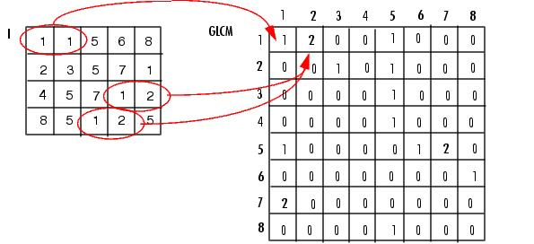
To create a GLCM, use the graycomatrix function. The graycomatrix function creates a gray-level co-occurrence matrix (GLCM) by calculating how often a pixel with the intensity (gray-level) value i occurs in a specific spatial relationship to a pixel with the value j. By default, the spatial relationship is defined as the pixel of interest and the pixel to its immediate right (horizontally adjacent), but you can specify other spatial relationships between the two pixels. Each element (i,j) in the resultant glcm is simply the sum of the number of times that the pixel with value i occurred in the specified spatial relationship to a pixel with value j in the input image.
Because the processing required to calculate a GLCM for the full dynamic range of an image is prohibitive, graycomatrix scales the input image. By default, graycomatrix uses scaling to reduce the number of intensity values in grayscale image from 256 to eight. The number of gray levels determines the size of the GLCM. To control the number of gray levels in the GLCM and the scaling of intensity values, using the NumLevels and the GrayLimits parameters of the graycomatrix function. See the graycomatrix reference page for more information.
The gray-level co-occurrence matrix can reveal certain properties about the spatial distribution of the gray levels in the texture image. For example, if most of the entries in the GLCM are concentrated along the diagonal, the texture is coarse with respect to the specified offset. You can also derive several statistical measures from the GLCM. See Deriving Statistics from a GLCM for more information.
To illustrate, the following figure shows how graycomatrix calculates the first three values in a GLCM. In the output GLCM, element (1,1) contains the value 1 because there is only one instance in the input image where two horizontally adjacent pixels have the values 1 and 1, respectively. glcm(1,2) contains the value 2 because there are two instances where two horizontally adjacent pixels have the values 1 and 2. Element (1,3) in the GLCM has the value 0 because there are no instances of two horizontally adjacent pixels with the values 1 and 3. graycomatrix continues processing the input image, scanning the image for other pixel pairs (i,j) and recording the sums in the corresponding elements of the GLCM.
Process Used to Create the GLCM
Specifying the Offsets
By default, the graycomatrix function creates a single GLCM, with the spatial relationship, or offset, defined as two horizontally adjacent pixels. However, a single GLCM might not be enough to describe the textural features of the input image. For example, a single horizontal offset might not be sensitive to texture with a vertical orientation. For this reason, graycomatrix can create multiple GLCMs for a single input image.
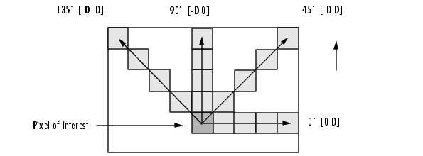
To create multiple GLCMs, specify an array of offsets to the graycomatrix function. These offsets define pixel relationships of varying direction and distance. For example, you can define an array of offsets that specify four directions (horizontal, vertical, and two diagonals) and four distances. In this case, the input image is represented by 16 GLCMs. When you calculate statistics from these GLCMs, you can take the average.
You specify these offsets as a p-by-2 array of integers. Each row in the array is a two-element vector, [row_offset, col_offset], that specifies one offset. row_offset is the number of rows between the pixel of interest and its neighbor. col_offset is the number of columns between the pixel of interest and its neighbor. This example creates an offset that specifies four directions and 4 distances for each direction. For more information about specifying offsets, see the graycomatrix reference page.
offsets = [ 0 1; 0 2; 0 3; 0 4;...
           -1 1; -2 2; -3 3; -4 4;...
           -1 0; -2 0; -3 0; -4 0;...
           -1 -1; -2 -2; -3 -3; -4 -4];
- The figure illustrates the spatial relationships of pixels that are defined by this array of offsets, where
Drepresents the distance from the pixel of interest.
Deriving Statistics from a GLCM
After you create the GLCMs, you can derive several statistics from them using the graycoprops function. These statistics provide information about the texture of an image. The following table lists the statistics you can derive. You specify the statistics you want when you call the graycoprops function. For detailed information about these statistics, see the graycoprops reference page.
Example: Plotting the Correlation
This example shows how to create a set of GLCMs and derive statistics from them and illustrates how the statistics returned by graycoprops have a direct relationship to the original input image.
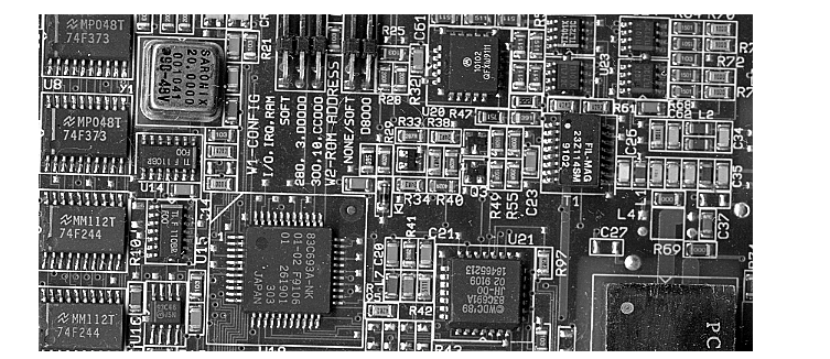
- Read in a grayscale image and display it. The example converts the truecolor image to a grayscale image and then rotates it 90° for this example.
- Define offsets of varying direction and distance. Because the image contains objects of a variety of shapes and sizes that are arranged in horizontal and vertical directions, the example specifies a set of horizontal offsets that only vary in distance.
- Create the GLCMs. Call the
graycomatrixfunction specifying the offsets. - Derive statistics from the GLCMs using the
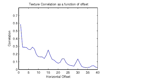
graycopropsfunction. The example calculates the contrast and correlation. - Plot correlation as a function of offset.
figure, plot([stats.Correlation]);
title('Texture Correlation as a function of offset');
xlabel('Horizontal Offset')
ylabel('Correlation')


The plot contains peaks at offsets 7, 15, 23, and 30. If you examine the input
image closely, you can see that certain vertical elements in the image have
a periodic pattern that repeats every seven pixels. The following figure
shows the upper left corner of the image and points out where this pattern
occurs.
 |
Using Texture Filter Functions | Intensity Adjustment |  |
© 1994-2005 The MathWorks, Inc.
'Digital Image Processing' 카테고리의 다른 글
| 17 Colors APIs (0) | 2017.07.27 |
|---|---|
| A simple C++ project for applying filters to raw images via command line. http://www.albertodebortoli.it (0) | 2017.03.13 |
| Embossing filter (0) | 2017.01.13 |
| Taking partial derivatives is easy in Matlab (0) | 2016.12.01 |
| Matlab Image Processing (0) | 2016.12.01 |


