


'Digital Image Processing > Course' 카테고리의 다른 글
| Introduction to Image Processing - 유튜브 동영상 강의 (0) | 2019.06.13 |
|---|
| Introduction to Image Processing - 유튜브 동영상 강의 (0) | 2019.06.13 |
|---|
| Digital Signal Processing - 유튜브 동영상 강의 (0) | 2019.06.13 |
|---|
Colors Apis
| Name | Description | Category | Date |
|---|---|---|---|
| Icons8 |
Icons8 provides an extensive ISO compliant icon library. The API allows developers to search and retrieve icons that can be used for template customization, build graphic and text editors, and to... | Images | 06.15.2017 |
| PrintCalc |
The PrintCalc API returns the percentage of a .pdf, .eps or .ps file's CMYK and Spot Color coverage. The API supports PDF, EPS, and PS files. HTTP POST is the preferred request method. The... | 04.01.2017 | |
| TinEye MulticolorEngine |
The TinEye MulticolorEngine API allows developers to make their image collections searchable by color. The API can extract color palettes from images, identify and search images by color, and support... | Search | 01.19.2017 |
| W3C CSS Painting |
The W3C CSS Painting API is a specification that describes an API for allowing developers to use an additional |
Images | 09.27.2016 |
| Image Color Extraction |
Use this HTTP/JSON API to extract colors from any image. The Image Color Extraction API can return colors in multiple formats, such as: RGB, HEX, HSL, HSB or RGBA. Sign up with Mashape to receive... | Colors | 02.18.2015 |
| Coinprism Colored Coins |
Coinprism is a service that allows for the tokenization of cryptocurrency. Using Coinprism's Colored Coins, users are able to trade shares, bonds, and commodities without regulation by coloring... | Bitcoin | 08.25.2014 |
| Croar.net RGB Picker |
Croar.net provides a simple RGB color picker widget that users can add to any webpage by inserting a few lines of JavaScript code. A demo of this widget is available with the documentation. The Croar... | Widgets | 01.02.2014 |
| APICloud.Me ColorTag |
APICloud.Me is a cloud-based API provider that aims to deliver scalable APIs that are simple to consume, reliable, and well documented. ColorTag is an API capable of detecting colors within an image... | Tools | 11.17.2013 |
| MyELearningSpace Web Accessibility |
The service provides review and validation of a website's accessibility for all users, including those with impaired eyesight, hearing, and motor skills. It helps designers to make content... | Colors | 07.23.2012 |
| Pictaculous |
Pictaculous is a color palette generator service from MailChimps. Users can upload PNG, GIF, or JPG image files and Pictaculous will analyze their colors to return a fitting scheme. Pictaculous'... | Tools | 05.07.2012 |
| AChecker |
The service provides analysis and validation of accessibility of web resources for users with disabilities. It can perform an automated review of resources at a specified URL, with a validation... | Colors | 03.02.2012 |
| Image Color Summarizer |
The web service provides statistics describing color characteristics of an image identified by URL. Summary data indicate the single RGB color that best represents the image, along with average hue... | Photos | 11.29.2011 |
| Colorfy It |
Colorfy It is a web application that lets users copy and paste website URLs into a box, and it returns the colors, CSS, and color ID information from the website for color analysis. The Colorfy It... | Colors | 10.11.2011 |
| Colr.org |
Colr.org is an online service that allows users to search for images, colors, and color schemes. Users can edit colors and color schemes, tag them, and download them. Users can also search for... | Other | 08.07.2011 |
| Empora Evergreen |
Fashion search API that returns clothes and accessories data based on search parameters including price, brand, color, and title/description. Developers can earn revenue when people click through to... | Search | 10.01.2010 |
| ColoRotate |
Bring 3D color into your web site or blog using the ColoRotate API. Use it to display palettes of color on your site in 3D, or create complex mashups. With the ColoRotate and JavaScript, you can get... | Tools | 05.29.2010 |
| COLOURlovers |
From their site: With the release of the COLOURlovers API, you can now access almost 1 million named colors and more than 325,000 color palettes for your creative projects and applications. Creating... | Tools | 04.20.2008 |
| A simple C++ project for applying filters to raw images via command line. http://www.albertodebortoli.it (0) | 2017.03.13 |
|---|---|
| Using a Gray-Level Co-Occurrence Matrix (GLCM) (0) | 2017.02.03 |
| Embossing filter (0) | 2017.01.13 |
| Taking partial derivatives is easy in Matlab (0) | 2016.12.01 |
| Matlab Image Processing (0) | 2016.12.01 |
Image Analysis Filters
A simple C++ project for applying filters to raw images via command line.
Author: Alberto De Bortoli
Date: august 2008
Course: Elaborazione delle Immagini (Image Analysis) Università degli studi di Padova, Prof. Paolo Cattani
Website: albertodebortoli.it
Compile the project with 'make' command with g++ (tested on version 4.2.1). Executable file 'ImageFilters' is generated for your architecture.
Source code files in the project:
The project implement the following:
Execution needs at least 7 command line arguments. 6 base arguments and 1 for the chosen filter to apply to the source image. First 6 base arguments are described as follow:
Here is an example of usage with the first 6 arguments:
./ImageFilters ./img/400x300RGB.raw ./img/output.raw 400 300 1 0
One more argument (at least) is needed for filter application. Filters can be applied sequentially. Filters description follows.
Spread the hystogram of gray over all the range of color space.
syntax: e
example: e
Modify the image brightness using a given value.
syntax: l <mod_value>
example: l 2.0
Apply auto contrast filter. Spread the hystogram to use the entire range.
syntax: a
example: a
Apply Gamma Correction filter with a given value.
syntax: g <mod_value>
example: g 0.8
Apply Gamma Correction filter on a given RGB channel with a given value. Only applicable to color images.
syntax: h <mod_value> <channel>
example: h 0.8 R
Invert the colors in the image.
syntax: i
example: i
Mirror the image. If <mod_value> is the direction ('X' for horizontally, 'Y' for vertically).
syntax: m <mod_value>
example: m X
Apply the pixelize filter. <mod_value> is the size of the macro pixel in the output image.
syntax: p <mod_value>
example: p 6
Apply smooth effect using a <kernel_dim>x<kernel_dim> kernel matrix.
syntax: s <kernel_dim>
example: s 5
Remove the noise using a <kernel_dim>x<kernel_dim> kernel matrix.
syntax: r <kernel_dim>
example: r 5
Apply a convolution filter using a 3x3 kernel matrix.< filter_type> can be:
'S' for Sharpen filter
'B' for Blur filter
'O' for Outliner (emboss filter)
syntax: c <filter_type>
example: c S
Rotate the image of degrees.
syntax: q <rotation_angle>
example: q 45
Zoom in or out. <zoom_flag> can be '-' for zoom in or '+' for zoom out. <mod_value> is the zoom percentage.
syntax: z <zoom_flag> <mod_value>
example: z + 30
Resize the image. Output image has width, height is proportionally derived. syntax: Z <mod_value>
example: Z 250
Convert a color image (RGB) to grayscale. Only applicable to grayscale images.
syntax: b
example: b
Cuts off high frequencies. <cutoff_value> (the cut off value) and <kernel_dim> (the kernel dimension) result in a stronger or weaker filter effect.
syntax: - <cutoff_value> <kernel_dim>
example: - 15 5
Two kind of Fourier Transform can be used: FT and FFT. They are used for frequency filtering (low-pass/high-pass filter). Classic FT runs in N^2, FFT runs in N log N.
syntax: <FT_type> <filter_type> <cutoff_value> <filtering_type>
example: f l 30 I
<FT_type> is for FT ('f') or for FFT ('F').
< filter_type> can be 'l' o 'h' based on low or high filter application.
< cutoff_value> is the cutoff value.
< filtering_type> is for ideal filtering (ILPF/IHPF) ('I') or bell shaped 'B' one.
Application of filter automatically saves spectrum in ‘magnitude.raw’ file for later access.
Here are example of usage of FT. Source image is 128x128 grayscale.
Original image
Transform spectrum
Here are the spectrums and the image as result of filter application.
Low-pass filter, ideal, threshold = 30
syntax: ./ImageFilters ./img/128x128BN.raw ./img/output.raw 128 128 0 0 F l 30 I
Low-pass filter, bell shaped, threshold = 30
syntax: ./ImageFilters ./img/128x128BN.raw ./img/output.raw 128 128 0 0 F l 30 C
High-pass filter, ideal, threshold = 10
syntax: ./ImageFilters ./img/128x128BN.raw ./img/output.raw 128 128 0 0 F h 10 I
High-pass filter, ideal, threshold = 10
syntax: ./ImageFilters ./img/128x128BN.raw ./img/output.raw 128 128 0 0 F h 10 C
Source images need to be power of 2 size to apply FFT. If not, scaling to next power of 2 is applied filling empty spaces with 0 (black). The image is then trimmed back to original size fter FFT.
Source image 160x100
Scaled image to power of 2 size, i.e 256x128
Scaled image spectrum
Image after backward FFT
Cut image to original size 160x100
Following images show the differences between hystogram equalization of pre and post equalization.

Pre filtering equalization

Post filtering equalization
Licensed under the New BSD License.
Copyright (c) 2008, Alberto De Bortoli at Università degli Studi di Padova. All rights reserved.
Redistribution and use in source and binary forms, with or without modification, are permitted provided that the following conditions are met: * Redistributions of source code must retain the above copyright notice, this list of conditions and the following disclaimer. * Redistributions in binary form must reproduce the above copyright notice, this list of conditions and the following disclaimer in the documentation and/or other materials provided with the distribution. * Neither the name of the Università degli Studi di Padova nor the names of its contributors may be used to endorse or promote products derived from this software without specific prior written permission.
THIS SOFTWARE IS PROVIDED BY Alberto De Bortoli ``AS IS'' AND ANY EXPRESS OR IMPLIED WARRANTIES, INCLUDING, BUT NOT LIMITED TO, THE IMPLIED WARRANTIES OF MERCHANTABILITY AND FITNESS FOR A PARTICULAR PURPOSE ARE DISCLAIMED. IN NO EVENT SHALL Alberto De Bortoli BE LIABLE FOR ANY DIRECT, INDIRECT, INCIDENTAL, SPECIAL, EXEMPLARY, OR CONSEQUENTIAL DAMAGES (INCLUDING, BUT NOT LIMITED TO, PROCUREMENT OF SUBSTITUTE GOODS OR SERVICES; LOSS OF USE, DATA, OR PROFITS; OR BUSINESS INTERRUPTION) HOWEVER CAUSED AND ON ANY THEORY OF LIABILITY, WHETHER IN CONTRACT, STRICT LIABILITY, OR TORT (INCLUDING NEGLIGENCE OR OTHERWISE) ARISING IN ANY WAY OUT OF THE USE OF THIS SOFTWARE, EVEN IF ADVISED OF THE POSSIBILITY OF SUCH DAMAGE.
| 17 Colors APIs (0) | 2017.07.27 |
|---|---|
| Using a Gray-Level Co-Occurrence Matrix (GLCM) (0) | 2017.02.03 |
| Embossing filter (0) | 2017.01.13 |
| Taking partial derivatives is easy in Matlab (0) | 2016.12.01 |
| Matlab Image Processing (0) | 2016.12.01 |
This is the html version of the file https://committee.tta.or.kr/include/Download.jsp?filename=choan%2F2012-1420+%B8%D6%C6%BC+%BD%BA%C5%D7%B7%B9%BF%C0+%B1%E2%B9%DD+%B0%ED%C1%A4+3D++%C6%E4%C0%CC%BC%C8+%BD%BA%C4%B3%B4%D7+%B9%E6%B9%FD_2%C2%F7%BC%F6%C1%A4%BA%BB.hwp.
완전 방사체인 흑체는 열을 가하면 금속과 같이 달궈지면서 붉은색을 띠다가 점차 밝은 흰색을 띠게 된다. 흑체는 속이 빈 뜨거운 공과 같으며 분광 에너지 분포가 물질의 구성이 아닌 온도에 의존하는 특징이 있다. 색온도는 온도가 높아지면 푸른색, 낮아지면 붉은색을 띤다. 우리가 주변에서 흔히 보는 태양광은 5,500∼7,000°K, 카메라 플래시는 5,600∼6,000°K, 백열등은 2,500∼3,600°K, 촛불은 1,800∼2,000°K가 된다.
| CIE standard illuminant (0) | 2017.02.14 |
|---|---|
| Automatic ColorChecker Detection, a Survey (0) | 2016.07.15 |
| Normalize colors under different lighting conditions (0) | 2016.05.31 |
| How to color correct an image from with a color checker (0) | 2016.05.30 |
| color correction with color checker - matlab code (0) | 2016.05.25 |
http://terms.naver.com/entry.nhn?docId=271066&cid=42641&categoryId=42641
국제 조명 위원회(Commission Internation ale de I'Eclair age: CIE)에서 정한 기준이 되는 광원.
국제적으로 정확한 색의 측정을 위해 사용된다. 국제 조명 위원회(CIE)에 의해서 분광 분포가 규정지어진 표준광은 A, B, C, D의 네 종류가 있다. CIE에서 규정한 측색용의 빛. 이에는 A, B, C, D가 있다.
(1) 표준광 A는 상관색온도가 약 2,856K인 완전 방사체가 발하는 빛으로 텅스텐 전구의 빛을 나타낸다.
(2) 표준광 B는 상관색온도가 약 4,874K인 가시 파장역의 직사 태양광을 나타내며 현재 거의 사용하지 않고 있다.
(3) 표준광 C는 상관색온도가 약 6,774K인 가시파장역의 평균적인 주광이다. 표준광 D65는 상관색온도가 약 6,504K인 자외선 영역을 포함한 평균적인 CIE 주광이다.
(4) 기타 표준광 D는 기타 상관색온도에서의 이 CIE 주광으로서 D65에 따른 것으로서는 표준광 D65(5,503K) 및 표준광 D75(7,504K)를 측색용 표준광으로 우선적으로 사용한다.

[네이버 지식백과] CIE 표준광 [CIE standard illuminant] (색채용어사전, 2007., 도서출판 예림)
http://www.ktword.co.kr/abbr_view.php?m_temp1=4526
1. 표준 광원 / 기준 광원 / 측색용 광원 (Standard Illuminant)
ㅇ 물체 색이 조명 종류 및 세기에 따라 달라지므로 이를 표준화하기 위한 조명 광원
- 상대 분광 전력 분포(relative spectral power distribution)로써 정의되는 광원
* (이를 물리적으로 굳이 나타낼 필요는 없음)
- 조명 광원 빛의 분광 분포가 변화하면,
. 이에따라 물체색의 삼자극치도 변화하므로,
. 객관적으로 색을 표시할 수 없으므로,
. 상대 분광 분포를 규정한 측색용의 표준 광원
2. 표준광원 종류
ㅇ 표준광원 A
- 가스 충전 상태의 텅스텐 백열 전구에 의한 조명시 색 묘사를 위함 (상관 색온도 2856 K)
. 2856 K의 흑체가 발하는 빛
ㅇ 표준광원 B
- 대낮 태양의 평균 직사량을 나타냄 (상관 색온도 4900 K)
. 현재는 사용하지 않음
ㅇ 표준광원 C
- 흐른 하늘 낮의 평균 직사량을 나타냄 (상관 색온도 6800 K)
. 표준광원 A에 데이비드-깁슨 필터(David-Gibson Filter)로 필터링하여 얻어지는 것
으로 엄밀성이 다소 결여됨
ㅇ 표준광원 D
- 실제 대낮의 태양광(자연 일광,daylight)을 측정하여 얻은 평균 데이터
. 표준광 C를 보완하고, 임의의 색온도를 조정한 것
- D50 : 정오의 태양광선을 대표적으로 묘사 (상관 색온도 5000 K)
- D55 : (상관 색온도 5500 K)
- D60 : 컴퓨터 그래픽 분야에서 많이 사용 (상관 색온도 6000 K)
- D65 : 북쪽하늘의 평균 태양광선을 대표적으로 묘사 (상관 색온도 6500 K)
. 페인트,플라스틱,직물 산업에서 주로 사용
. 표준광 C에 비해 자외선 영역의 단파장 빛이 강함
- D75 : 북쪽하늘의 태양광선을 대표적으로 묘사 (상관 색온도 7500 K)
ㅇ 표준광원 E
- 이론적으로 동일한 에너지를 갖음
- 실제 광원이 아닌 주로 계산 목적으로 사용됨
ㅇ 표준광원 F 시리즈
- 일반적인 형광등 광 수준
- F2 ~ F12
※ [참고_웹]
- 표준광원 분광분포(Spectral Distribution) 그림 例 : A,C,D26 분광분포도
- 복사측정 표준: 자외선부터 적외선까지
- 표준광원의 이해와 측색 조명환경
3. 주요 표준광 분류
ㅇ CIE 분류 표준광 : A, C, D50, D65, F2, F8, F11 등
ㅇ 한국산업규격(KS A0074) 분류 표준광
- 표준광 A, C, D65
- 보조표준광 B, D50, D55, D75
- 시료광 F6, F8, F10
| 카메라 플래시 색 온도 (0) | 2017.02.14 |
|---|---|
| Automatic ColorChecker Detection, a Survey (0) | 2016.07.15 |
| Normalize colors under different lighting conditions (0) | 2016.05.31 |
| How to color correct an image from with a color checker (0) | 2016.05.30 |
| color correction with color checker - matlab code (0) | 2016.05.25 |
http://sijoo.tistory.com/90
| Image Processing Toolbox User's Guide |   |
Using a Gray-Level Co-Occurrence Matrix (GLCM)
The texture filter functions provide a statistical view of texture based on the image histogram. These functions can provide useful information about the texture of an image but cannot provide information about shape, i.e., the spatial relationships of pixels in an image.
Another statistical method that considers the spatial relationship of pixels is the gray-level co-occurrence matrix (GLCM), also known as the gray-level spatial dependence matrix. The toolbox provides functions to create a GLCM and derive statistical measurements from it.
This section includes the following topics.
Creating a Gray-Level Co-Occurrence Matrix
To create a GLCM, use the graycomatrix function. The graycomatrix function creates a gray-level co-occurrence matrix (GLCM) by calculating how often a pixel with the intensity (gray-level) value i occurs in a specific spatial relationship to a pixel with the value j. By default, the spatial relationship is defined as the pixel of interest and the pixel to its immediate right (horizontally adjacent), but you can specify other spatial relationships between the two pixels. Each element (i,j) in the resultant glcm is simply the sum of the number of times that the pixel with value i occurred in the specified spatial relationship to a pixel with value j in the input image.
Because the processing required to calculate a GLCM for the full dynamic range of an image is prohibitive, graycomatrix scales the input image. By default, graycomatrix uses scaling to reduce the number of intensity values in grayscale image from 256 to eight. The number of gray levels determines the size of the GLCM. To control the number of gray levels in the GLCM and the scaling of intensity values, using the NumLevels and the GrayLimits parameters of the graycomatrix function. See the graycomatrix reference page for more information.
The gray-level co-occurrence matrix can reveal certain properties about the spatial distribution of the gray levels in the texture image. For example, if most of the entries in the GLCM are concentrated along the diagonal, the texture is coarse with respect to the specified offset. You can also derive several statistical measures from the GLCM. See Deriving Statistics from a GLCM for more information.
To illustrate, the following figure shows how graycomatrix calculates the first three values in a GLCM. In the output GLCM, element (1,1) contains the value 1 because there is only one instance in the input image where two horizontally adjacent pixels have the values 1 and 1, respectively. glcm(1,2) contains the value 2 because there are two instances where two horizontally adjacent pixels have the values 1 and 2. Element (1,3) in the GLCM has the value 0 because there are no instances of two horizontally adjacent pixels with the values 1 and 3. graycomatrix continues processing the input image, scanning the image for other pixel pairs (i,j) and recording the sums in the corresponding elements of the GLCM.
Process Used to Create the GLCM
Specifying the Offsets
By default, the graycomatrix function creates a single GLCM, with the spatial relationship, or offset, defined as two horizontally adjacent pixels. However, a single GLCM might not be enough to describe the textural features of the input image. For example, a single horizontal offset might not be sensitive to texture with a vertical orientation. For this reason, graycomatrix can create multiple GLCMs for a single input image.
To create multiple GLCMs, specify an array of offsets to the graycomatrix function. These offsets define pixel relationships of varying direction and distance. For example, you can define an array of offsets that specify four directions (horizontal, vertical, and two diagonals) and four distances. In this case, the input image is represented by 16 GLCMs. When you calculate statistics from these GLCMs, you can take the average.
You specify these offsets as a p-by-2 array of integers. Each row in the array is a two-element vector, [row_offset, col_offset], that specifies one offset. row_offset is the number of rows between the pixel of interest and its neighbor. col_offset is the number of columns between the pixel of interest and its neighbor. This example creates an offset that specifies four directions and 4 distances for each direction. For more information about specifying offsets, see the graycomatrix reference page.
offsets = [ 0 1; 0 2; 0 3; 0 4;...
           -1 1; -2 2; -3 3; -4 4;...
           -1 0; -2 0; -3 0; -4 0;...
           -1 -1; -2 -2; -3 -3; -4 -4];
D represents the distance from the pixel of interest.
Deriving Statistics from a GLCM
After you create the GLCMs, you can derive several statistics from them using the graycoprops function. These statistics provide information about the texture of an image. The following table lists the statistics you can derive. You specify the statistics you want when you call the graycoprops function. For detailed information about these statistics, see the graycoprops reference page.
Example: Plotting the Correlation
This example shows how to create a set of GLCMs and derive statistics from them and illustrates how the statistics returned by graycoprops have a direct relationship to the original input image.
graycomatrix function specifying the offsets. graycoprops function. The example calculates the contrast and correlation. figure, plot([stats.Correlation]); title('Texture Correlation as a function of offset'); xlabel('Horizontal Offset') ylabel('Correlation') The plot contains peaks at offsets 7, 15, 23, and 30. If you examine the input image closely, you can see that certain vertical elements in the image have a periodic pattern that repeats every seven pixels. The following figure shows the upper left corner of the image and points out where this pattern occurs.
| |
Using Texture Filter Functions | Intensity Adjustment | |
© 1994-2005 The MathWorks, Inc.
| 17 Colors APIs (0) | 2017.07.27 |
|---|---|
| A simple C++ project for applying filters to raw images via command line. http://www.albertodebortoli.it (0) | 2017.03.13 |
| Embossing filter (0) | 2017.01.13 |
| Taking partial derivatives is easy in Matlab (0) | 2016.12.01 |
| Matlab Image Processing (0) | 2016.12.01 |
#define emboss_w 3
#define emboss_h 3

sumr=0;
sumg=0;
sumb=0;

int emboss_filter[emboss_w][emboss_h]={{2,0,0},{0,-1,0},{0,0,-1}};
int emboss_sum=1;

for(i=1;i<temp->w-1;i++){
  for(j=1;j<temp->h-1;j++){
    color=getpixel(temp,i,j);
    r=getr32(color);
    g=getg32(color);
    b=getb32(color);
    h=(r+g+b)/3;
    if(h>255)
      h=255;
    if(h<0)
      h=0;
    putpixel(temp1,i,j,makecol(h,h,h));
  }
}

for(i=1;i<temp->w-1;i++){
  for(j=1;j<temp->h-1;j++){
    sumr=0;
    for(k=0;k<emboss_w;k++){
      for(l=0;l<emboss_h;l++){
        color=getpixel(temp1,i-((emboss_w-1)>>1)+k,j-((
        emboss_h-1)>>1)+l);
        r=getr32(color);
        sumr+=r*emboss_filter[k][l];
      }
    }
    sumr/=emboss_sum;
    sumr+=128;
    if(sumr>255)
      sumr=255;
    if(sumr<0)
      sumr=0;
    putpixel(temp2,i,j,makecol(sumr,sumr,sumr));
  }
}
Here are the effects of this algorithm:
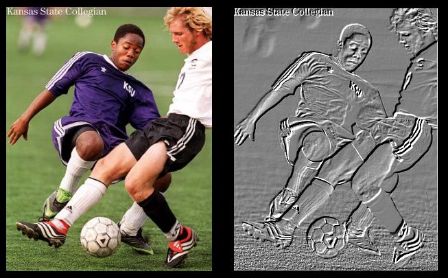
Picture 9: Embossing filter
| A simple C++ project for applying filters to raw images via command line. http://www.albertodebortoli.it (0) | 2017.03.13 |
|---|---|
| Using a Gray-Level Co-Occurrence Matrix (GLCM) (0) | 2017.02.03 |
| Taking partial derivatives is easy in Matlab (0) | 2016.12.01 |
| Matlab Image Processing (0) | 2016.12.01 |
| Gabor Filter 이해하기 (0) | 2016.10.17 |
Taking partial derivatives is easy in Matlab ( also why I don't like the class uint8 )

| Using a Gray-Level Co-Occurrence Matrix (GLCM) (0) | 2017.02.03 |
|---|---|
| Embossing filter (0) | 2017.01.13 |
| Matlab Image Processing (0) | 2016.12.01 |
| Gabor Filter 이해하기 (0) | 2016.10.17 |
| identify the redness (0) | 2016.05.11 |
– Scroll below: Learn Matlab function for active contours.
Active Contours in Matlab (Image Processing):
* Inbuilt Matlab functions have been made use of in implementing the
  below code.
close all
clear all
clc

% read the input image
inpImage =imread('coin_1.jpg');
% size of image
[rows cols dims] = size(inpImage);

if dims==3
    inpImage=double(rgb2gray(inpImage));
else
    inpImage=double(inpImage);
end

% Gaussian filter parameter
sigma=1.2;
% Gaussian filter
G=fspecial('gaussian',15,sigma);
% Gaussian smoothed image
inpImage=conv2(inpImage,G,'same');


% gradient of image
[gradIX,gradIY]=gradient(inpImage);
absGradI=sqrt(gradIX.^2+gradIY.^2);


% higher dimensional embedding function phi whose zero level set is our
% contour
% radius of circle - initial embedding function
% radius=min(floor(0.45*rows),floor(0.45*cols));
[u,v] = meshgrid(1:cols, 1:rows);
phi = ((u-cols/2)/(floor(0.45*cols))).^2+((v-rows/2)/(floor(0.45*rows))).^2-1;

% edge-stopping function
g = 1./(1+absGradI.^2);
% gradient of edge-stopping function
[gx,gy]=gradient(g);

% gradient descent step size
dt=.4;

% number of iterations after which we reinitialize the surface
num_reinit=10;

phiOld=zeros(rows,cols);

% number of iterations
iter=0;

while(sum(sum(abs(phi-phiOld)))~=0)
    % gradient of phi
    [gradPhiX gradPhiY]=gradient(phi);
    % magnitude of gradient of phi
    absGradPhi=sqrt(gradPhiX.^2+gradPhiY.^2);
    % normalized gradient of phi - eliminating singularities
    normGradPhiX=gradPhiX./(absGradPhi+(absGradPhi==0));
    normGradPhiY=gradPhiY./(absGradPhi+(absGradPhi==0));

    [divXnormGradPhiX divYnormGradPhiX]=gradient(normGradPhiX);
    [divXnormGradPhiY divYnormGradPhiY]=gradient(normGradPhiY);
    % curvature is the divergence of normalized gradient of phi
    K = divXnormGradPhiX + divYnormGradPhiY;
    % dPhiBydT
    dPhiBydT =( g.*K.*absGradPhi + g.*absGradPhi + (gx.*gradPhiX+gy.*gradPhiY) );
    phiOld=phi;
    % level set evolution equation
    phi = phi + ( dt * dPhiBydT );
    iter=iter+1;
    if mod(iter,num_reinit)==0
        % reinitialize the embedding function after num_reinit iterations
        phi=sign(phi);
        phi = double((phi > 0).*(bwdist(phi < 0)) - (phi < 0).*(bwdist(phi > 0)));
    end
    if mod(iter,10)==0
        pause(0.05)
        iter
        imagesc(inpImage)
        colormap(gray)
        hold on
        contour(phi,[0 0],'r')
        %         close all
        %         surf(phi)
        %         pause
    end
end
This demo shows how a image looks like after thresholding. The percentage of the thresholding means the threshold level between the maximum and minimum indesity of the initial image. Thresholding is a way to get rid of the effect of noise and to improve the signal-noise ratio. That is, it is a way to keep the significant imformation of the image while get rid of the unimportant part (under the condition that you choose a plausible thresholding level). In the Canny edge detector part, you will see that, before thinning, we first do some thresholding. You are encouraged to do thinning without thresholding and to see what is the advantage of thresholding.
| lena.gif | 10% threshold |
|---|---|
 |
 |
| 20% threshold | 30% threshold |
|---|---|
 |
 |
This program show the effect of thresholding. The output are four subfigures shown in the same figure:
The MATLAB codes:
%%%%%%%%%%%%% The main.m file %%%%%%%%%%%%%%
clear;
% Threshold level parameter alfa:
alfa=0.1;% less than 1/3

[x,map]=gifread('lena.gif');
ix=ind2gray(x,map);
I_max=max(max(ix));
I_min=min(min(ix));
level1=alfa*(I_max-I_min)+I_min;
level2=2*level1;
level3=3*level1;
thix1=max(ix,level1.*ones(size(ix)));
thix2=max(ix,level2.*ones(size(ix)));
thix3=max(ix,level3.*ones(size(ix)));
figure(1);colormap(gray);
subplot(2,2,1);imagesc(ix);title('lena');
subplot(2,2,2);imagesc(thix1);title('threshold one alfa');
subplot(2,2,3);imagesc(thix2);title('threshold two alfa');
subplot(2,2,4);imagesc(thix3);title('threshold three alfa');
%%%%%%%%%%%%% End of the main.m file %%%%%%%%%%%%%%
These demos show the basic effects of the (2D) Gaussian filter: smoothing the image and wiping off the noise. Generally speaking, for a noise-affected image, smoothing it by Gaussian function is the first thing to do before any other further processing, such as edge detection. The effectiveness of the gaussian function is different for different choices of the standard deviation sigma of the Gaussian filter. You can see this from the following demos.
| lena.gif | filtered with sigma = 3 | filtered with sigma = 1 |
|---|---|---|
| |
 |
 |
| noisy lena | filtered with sigma = 3 | filtered with sigma =1 |
|---|---|---|
 |
 |
 |
(Noise is generated by matlab function 0.3*randn(512))
This program show the effect of Gaussian filter. The output are four subfigures shown in the same figure:
The matlab codes:
%%%%%%%%%%%%% The main.m file  %%%%%%%%%%%%%%%
clear;
% Parameters of the Gaussian filter:
n1=10;sigma1=3;n2=10;sigma2=3;theta1=0;
% The amplitude of the noise:
noise=0.1;

[w,map]=gifread('lena.gif');
x=ind2gray(w,map);
filter1=d2gauss(n1,sigma1,n2,sigma2,theta);
x_rand=noise*randn(size(x));
y=x+x_rand;
f1=conv2(x,filter1,'same');
rf1=conv2(y,filter1,'same');
figure(1);
subplot(2,2,1);imagesc(x);
subplot(2,2,2);imagesc(y);
subplot(2,2,3);imagesc(f1);
subplot(2,2,4);imagesc(rf1);
colormap(gray);
%%%%%%%%%%%%%% End of the main.m file %%%%%%%%%%%%%%%


%%%%%%% The functions used in the main.m file %%%%%%%
% Function "d2gauss.m":
% This function returns a 2D Gaussian filter with size n1*n2; theta is
% the angle that the filter rotated counter clockwise; and sigma1 and sigma2
% are the standard deviation of the gaussian functions.
function h = d2gauss(n1,std1,n2,std2,theta)
r=[cos(theta) -sin(theta);
   sin(theta)  cos(theta)];
for i = 1 : n2
    for j = 1 : n1
        u = r * [j-(n1+1)/2 i-(n2+1)/2]';
        h(i,j) = gauss(u(1),std1)*gauss(u(2),std2);
    end
end
h = h / sqrt(sum(sum(h.*h)));

% Function "gauss.m":
function y = gauss(x,std)
y = exp(-x^2/(2*std^2)) / (std*sqrt(2*pi));
%%%%%%%%%%%%%% end of the functions %%%%%%%%%%%%%%%%
There are some results of applying Canny edge detector to real image (The black and white image “lena.gif” we used here was obtained by translating from a color lena.tiff using matlab. So it might not be the standard BW “lena”.) The thresholding parameter alfa is fix as 0.1. The size of the filters is also fixed as 10*10.
These images are all gray images though they might seem a little strange in your browser. To see them more clearly, just click these images and you will find the difference especially from the “result images”, that is, the titled “after thinning” ones. The safe way to see the correct display of these images is to grab these images and show them by “xv” or “matlab”. While, you are encouraged to use the given matlab codes and get these images in matlab by yourself. Try to change the parameters to get more sense about how these parameters affect the edge detection.
| lena.gif | vertical edges | horizontal edges |
|---|---|---|
| |
 |
 |
| norm of the gradient | after thresholding | after thinning |
|---|---|---|
 |
 |
 |
| lena.gif | vertical edges | horizontal edges |
|---|---|---|
| |
 |
 |
| norm of the gradient | after thresholding | after thinning |
|---|---|---|
 |
 |
 |
This part gives the algorithm of Canny edge detector. The outputs are six subfigures shown in the same figure:
The matlab codes:
%%%%%%%%%%%%% The main.m file  %%%%%%%%%%%%%%%
clear;
% The algorithm parameters:
% 1. Parameters of edge detecting filters:
%    X-axis direction filter:
     Nx1=10;Sigmax1=1;Nx2=10;Sigmax2=1;Theta1=pi/2;
%    Y-axis direction filter:
     Ny1=10;Sigmay1=1;Ny2=10;Sigmay2=1;Theta2=0;
% 2. The thresholding parameter alfa:
     alfa=0.1;

% Get the initial image lena.gif
[x,map]=gifread('lena.gif');
w=ind2gray(x,map);
figure(1);colormap(gray);
subplot(3,2,1);
imagesc(w,200);
title('Image: lena.gif');

% X-axis direction edge detection
subplot(3,2,2);
filterx=d2dgauss(Nx1,Sigmax1,Nx2,Sigmax2,Theta1);
Ix= conv2(w,filterx,'same');
imagesc(Ix);
title('Ix');

% Y-axis direction edge detection
subplot(3,2,3)
filtery=d2dgauss(Ny1,Sigmay1,Ny2,Sigmay2,Theta2);
Iy=conv2(w,filtery,'same');
imagesc(Iy);
title('Iy');

% Norm of the gradient (Combining the X and Y directional derivatives)
subplot(3,2,4);
NVI=sqrt(Ix.*Ix+Iy.*Iy);
imagesc(NVI);
title('Norm of Gradient');

% Thresholding
I_max=max(max(NVI));
I_min=min(min(NVI));
level=alfa*(I_max-I_min)+I_min;
subplot(3,2,5);
Ibw=max(NVI,level.*ones(size(NVI)));
imagesc(Ibw);
title('After Thresholding');

% Thinning (Using interpolation to find the pixels where the norms of
% gradient are local maximum.)
subplot(3,2,6);
[n,m]=size(Ibw);
for i=2:n-1,
for j=2:m-1,
 if Ibw(i,j) > level,
 X=[-1,0,+1;-1,0,+1;-1,0,+1];
 Y=[-1,-1,-1;0,0,0;+1,+1,+1];
 Z=[Ibw(i-1,j-1),Ibw(i-1,j),Ibw(i-1,j+1);
    Ibw(i,j-1),Ibw(i,j),Ibw(i,j+1);
    Ibw(i+1,j-1),Ibw(i+1,j),Ibw(i+1,j+1)];
 XI=[Ix(i,j)/NVI(i,j), -Ix(i,j)/NVI(i,j)];
 YI=[Iy(i,j)/NVI(i,j), -Iy(i,j)/NVI(i,j)];
 ZI=interp2(X,Y,Z,XI,YI);
  if Ibw(i,j) >= ZI(1) & Ibw(i,j) >= ZI(2)
  I_temp(i,j)=I_max;
  else
  I_temp(i,j)=I_min;
  end
 else
 I_temp(i,j)=I_min;
 end
end
end
imagesc(I_temp);
title('After Thinning');
colormap(gray);
%%%%%%%%%%%%%% End of the main.m file %%%%%%%%%%%%%%%


%%%%%%% The functions used in the main.m file %%%%%%%
% Function "d2dgauss.m":
% This function returns a 2D edge detector (first order derivative
% of 2D Gaussian function) with size n1*n2; theta is the angle that
% the detector rotated counter clockwise; and sigma1 and sigma2 are the
% standard deviation of the gaussian functions.
function h = d2dgauss(n1,sigma1,n2,sigma2,theta)
r=[cos(theta) -sin(theta);
   sin(theta)  cos(theta)];
for i = 1 : n2
    for j = 1 : n1
        u = r * [j-(n1+1)/2 i-(n2+1)/2]';
        h(i,j) = gauss(u(1),sigma1)*dgauss(u(2),sigma2);
    end
end
h = h / sqrt(sum(sum(abs(h).*abs(h))));

% Function "gauss.m":
function y = gauss(x,std)
y = exp(-x^2/(2*std^2)) / (std*sqrt(2*pi));

% Function "dgauss.m"(first order derivative of gauss function):
function y = dgauss(x,std)
y = -x * gauss(x,std) / std^2;
%%%%%%%%%%%%%% end of the functions %%%%%%%%%%%%%
——————————————————————————————————————————————-
Recall the wagon wheel test image used in the resampling example:
Marr/Hildreth edge detection is based on the zero-crossings of the Laplacian of the Gaussian operator applied to the image for various values of sigma, the standard deviation of the Gaussian. What follows is a mosaic of zero-crossings for four choices of sigma computed using the Matlab image processing toolbox. The top left is sigma=1, the top right is sigma=2, the bottom left is sigma=3 and the bottom right is sigma=4. (Matlab Laplacian of Gaussian edge detection normally selects a threshold so that only zero-crossings of sufficient strength are shown. Here, the threshold is forced to be zero so that all zero-crossings are reported, as is required by the Marr/Hildreth theory of edge detection.)
As most commonly implemented, Canny edge detection is based on extrema of the first derivative of the Gaussian operator applied to the image for various values of sigma, the standard deviation of the Gaussian. What follows is a mosaic of edge points for four choices of sigma computed using the Matlab image processing toolbox. The top left is sigma=1, the top right is sigma=2, the bottom left is sigma=3 and the bottom right is sigma=4. The Canny method uses two thresholds to link edge points. The Matlab implementation can estimate both thesholds automatically. For this example, I found the Matlab estimated thresholds to be somewhat conservative. Therefore, for the mosaic, I reduced the thresholds to 75 percent of their automatically estimated values.
You should observe that zero-crossings in Marr/Hildreth edge detection always form connected, closed contours (or leave the edge of the image). This comes, however, at the expense of localization, especially for larger values of sigma. Arguably, Canny edge detection does a better job of localization. Alas, with Canny edge detection, the edge segments can become disconnected
%    Image Processing Toolbox Version 5.4(R2007a)

A = imread('/ai/woodham/public_html/cpsc505/images/wheel.tif');

% Marr/Hildreth edge detection
% with threshold forced to zero
MH1 = edge(A,'log',0,1.0);
MH2 = edge(A,'log',0,2.0);
MH3 = edge(A,'log',0,3.0);
MH4 = edge(A,'log',0,4.0);

% form mosaic
EFGH = [ MH1 MH2; MH3 MH4];

%% show mosaic in Matlab Figure window
%log = figure('Name','Marr/Hildreth: UL: s=1  UR: s=2  BL: s=3 BR: s=4');
%iptsetpref('ImshowBorder','tight');
%imshow(EFGH,'InitialMagnification',100);

% Canny edge detection
[C1, Ct1] = edge(A,'canny',[],1.0);
[C2, Ct2] = edge(A,'canny',[],2.0);
[C3, Ct3] = edge(A,'canny',[],3.0);
[C4, Ct4] = edge(A,'canny',[],4.0);

% Recompute lowering both automatically computed
% thresholds by fraction k
k = 0.75
C1 = edge(A,'canny',k*Ct1,1.0);
C2 = edge(A,'canny',k*Ct2,2.0);
C3 = edge(A,'canny',k*Ct3,3.0);
C4 = edge(A,'canny',k*Ct4,4.0);

% form mosaic
ABCD= [ C1 C2; C3 C4 ];

% show mosaic in Matlab Figure window
%canny = figure('Name','Canny: UL: s=1  UR: s=2  BL: s=3 BR: s=4');
%iptsetpref('ImshowBorder','tight');
%imshow(ABCD,'InitialMagnification',100);

% write results to file
% Note: Matlab no longer reads/writes GIF files, owing to licence
%       restrictions.  Translation from TIF to GIF was done
%       manually (with xv) for inclusion in the web example page
imwrite(ABCD,'/ai/woodham/World/cpsc505/images/canny.tif','tif
imwrite(EFGH,'/ai/woodham/World/cpsc505/images/log.tif','tif
| Using a Gray-Level Co-Occurrence Matrix (GLCM) (0) | 2017.02.03 |
|---|---|
| Embossing filter (0) | 2017.01.13 |
| Taking partial derivatives is easy in Matlab (0) | 2016.12.01 |
| Gabor Filter 이해하기 (0) | 2016.10.17 |
| identify the redness (0) | 2016.05.11 |
영상처리에서 Bio-inspired라는 키워드가 있으면 빠지지않고 등장하는 Gabor Filter. 외곽선을 검출하는 기능을 하는 필터로, 사람의 시각체계가 반응하는 것과 비슷하다는 이유로 널리 사용되고 있다. Gabor Fiter는 간단히 말해서 사인 함수로 모듈레이션 된 Gaussian Filter라고 생각할 수 있다. 파라미터를 조절함에 따라 Edge의 크기나 방향성을 바꿀 수 있으므로 Bio-inspired 영상처리 알고리즘에서 특징점 추출 알고리즘으로 핵심적인 역할을 하고 있다.
2D Gabor Filter의 수식은 아래와 같다.

위에서와 같이 5개의 파라미터를 조절해서 사용할 수 있다. 복잡해보이는 파라미터들의 의미를 Filter Kernel을 JET Color Mapping한 이미지와 함께 직관적으로 이해해보자. (JET Color Mapping은 실제 Kernel 값을 기반으로 했으며, 사이즈만 가로, 가로 4배씩 Lienar Interpolation하였다.) Parameter를 나타내는 순서는 (σ,θ,λ,γ,ψ)다.


| Using a Gray-Level Co-Occurrence Matrix (GLCM) (0) | 2017.02.03 |
|---|---|
| Embossing filter (0) | 2017.01.13 |
| Taking partial derivatives is easy in Matlab (0) | 2016.12.01 |
| Matlab Image Processing (0) | 2016.12.01 |
| identify the redness (0) | 2016.05.11 |
https://ryanfb.github.io/etc/2015/07/08/automatic_colorchecker_detection.html
 https_ryanfb.github.io_etc_2015_07_08_automatic_colorchecker_.pdf
/etcryanfb.github.io
↳ Automatic ColorChecker Detection, a Survey
A while back (July 2010 going by Git commit history), I hacked together a program for automatically finding the GretagMacbeth ColorCheckerin an image, and cheekily named it Macduff.
The algorithm I developed used adaptive thresholding against the RGB channel images, followed by contour findingwith heuristics to try to filter down to ColorChecker squares, then using k-means clustering to cluster squares (in order to handle the case of images with an X-Rite ColorChecker Passport), then computing the average square colors and trying to find if any layout/orientation of square clusters would match ColorChecker reference values (within some Euclidean distance in RGB space). Because of the original use case I was developing this for (automatically calibrating images against an image of a ColorChecker on a copy stand), I could assume that the ColorChecker would take up a relatively large portion of the input image, and coded Macduff using this assumption.
I recently decided to briefly revisit this problem and see if any additional work had been done, and I thought a quick survey of what I turned up might be generally useful:
•Jackowski, Marcel, et al. Correcting the geometry and color of digital images. Pattern Analysis and Machine Intelligence, IEEE Transactions on 19.10 (1997): 1152-1158. Requires manual selection of patch corners, which are then refined with template matching.
•Tajbakhsh, Touraj, and Rolf-Rainer Grigat. Semiautomatic color checker detection in distorted images. Proceedings of the Fifth IASTED International Conference on Signal Processing, Pattern Recognition and Applications. ACTA Press, 2008. Unfortunately I cannot find any online full-text of this article, and my library doesn’t have the volume. Based on the description in Ernst 2013, the algorithm proceeds as follows: “The user initially selects the four chart corners in the image and the system estimates the position of all color regions using projective geometry. They transform the image with
a Sobel kernel, a morphological operator and thresholding into a binary image and find connected regions.”
•Kapusi, Daniel, et al. Simultaneous geometric and colorimetric camera calibration. 2010. This method requires color reference circles placed in the middle of black and white chessboard squares, which they then locate using OpenCV’s chessboard detection.
•Bianco, Simone, and Claudio Cusano. Color target localization under varying illumination conditions. Computational Color Imaging. Springer Berlin Heidelberg, 2011. 245-255. Uses SIFTfeature matching, and then clusters matched features to be fed into a pose selection and appearance validation algorithm.
•Brunner, Ralph T., and David Hayward. Automatic detection of calibration charts in images. Apple Inc., assignee. Patent US8073248. 6 Dec. 2011. Uses a scan-line based method to try to fit a known NxM reference chart.
•Minagawa, Akihiro, et al. A color chart detection method for automatic color correction. 21st International Conference on Pattern Recognition (ICPR). IEEE, 2012. Uses pyramidizationto feed a pixel-spotting algorithm which is then used for patch extraction.
•K. Hirakawa, “ColorChecker Finder,” accessed from http://campus.udayton.edu/~ISSL/software. AKA CCFind.m. The earliest Internet Archive Wayback Machine snapshotfor this page is in August 2013, however I also found this s-colorlab mailing list announcement from May 2012. Unfortunately this code is under a restrictive license: “This code is copyrighted by PI Keigo Hirakawa. The softwares are for research use only. Use of software for commercial purposes without a prior agreement with the authors is strictly prohibited.” According to the webpage, “CCFind.mdoes not detect squares explicitly. Instead, it learns the recurring shapes inside an image.”
•Liu, Mohan, et al. A new quality assessment and improvement system for print media. EURASIP Journal on Advances in Signal Processing 2012.1 (2012): 1-17. An automatic ColorChecker detection is described as part of a comprehensive system for automatic color correction. The algorithm first quantizes all colors to those in the color chart, then performs connected component analysis with heuristics to locate patch candidates, which are then fed to a Delaunay triangulation which is pruned to find the final candidate patches, which is then checked for the correct color orientation. This is the same system described in: Konya, Iuliu Vasile, and Baia Mare. Adaptive Methods for Robust Document Image Understanding. Diss. Universitäts-und Landesbibliothek Bonn, 2013.
•Devic, Goran, and Shalini Gupta. Robust Automatic Determination and Location of Macbeth Color Checker Charts. Nvidia Corporation, assignee. Patent US20140286569. 25 Sept. 2014. Uses edge-detection, followed by a flood-fill, with heuristics to try to detect the remaining areas as ColorChecker(s).
•Ernst, Andreas, et al. Check my chart: A robust color chart tracker for colorimetric camera calibration. Proceedings of the 6th International Conference on Computer Vision/Computer Graphics Collaboration Techniques and Applications. ACM, 2013. Extracts polygonal image regions and applies a cost function to check adaptation to a color chart.
•Kordecki, Andrzej, and Henryk Palus. Automatic detection of color charts in images. Przegląd Elektrotechniczny 90.9 (2014): 197-202. Uses image binarization and patch grouping to construct bounding parallelograms, then applies heuristics to try to determine the types of color charts.
•Wang, Song, et al. A Fast and Robust Multi-color Object Detection Method with Application to Color Chart Detection. PRICAI 2014: Trends in Artificial Intelligence. Springer International Publishing, 2014. 345-356. Uses per-channel feature extraction with a sliding rectangle, fed into a rough detection step with predefined 2x2 color patch templates, followed by precise detection.
•García Capel, Luis E., and Jon Y. Hardeberg. Automatic Color Reference Target Detection(Direct PDF link). Color and Imaging Conference. Society for Imaging Science and Technology, 2014. Implements a preprocessing step for finding an approximate ROI for the ColorChecker, and examines the effect of this for both CCFindand a template matching approach (inspired by a project report which I cannot locate online). They also make their software available for download at http://www.ansatt.hig.no/rajus/colorlab/CCDetection.zip.
Data Sets
•Colourlab Image Database: Imai’s ColorCheckers (CID:ICC)(246MB) Used by García Capel 2014. 43 JPEG images.
•Gehler’s Dataset(approx. 8GB, 592MB downsampled) ◦Shi’s Re-processing of Gehler’s Raw Dataset(4.2GB total) Used by Hirakawa. 568 PNG images.
◦Reprocessed Gehler“We noticed that the renderings provided by Shi and Funt made the colours look washed out. There also seemed to be a strong Cyan tint to all of the images. Therefore, we processed the RAW files ourselves using DCRAW. We followed the same methodology as Shi and Funt. The only difference is we did allow DCRAW to apply a D65 Colour Correction matrix to all of the images. This evens out the sensor responses.”
Originally published on 2015-07-08 by Ryan BaumannFeedback? e-mail/ twitter/ github
Revision History
Suggested citation:
Baumann, Ryan. “Automatic ColorChecker Detection, a Survey.” Ryan Baumann - /etc(blog), 08 Jul 2015, https://ryanfb.github.io/etc/2015/07/08/automatic_colorchecker_detection.html(accessed 15 Jul 2016).
Creative Commons License
This work is licensed under a Creative Commons Attribution 4.0 International License.
| 카메라 플래시 색 온도 (0) | 2017.02.14 |
|---|---|
| CIE standard illuminant (0) | 2017.02.14 |
| Normalize colors under different lighting conditions (0) | 2016.05.31 |
| How to color correct an image from with a color checker (0) | 2016.05.30 |
| color correction with color checker - matlab code (0) | 2016.05.25 |
I have done an outdoor experiment of a camera capturing images every 1 hour for color checker chart. I am trying to normalize each color so it looks the same through the day; as the color constancy is intensity independent.
I have tried several methods but the results were disappointing. Any ideas?
Thanks
---------------------------------------------------------------------------------------------
What methods did you try? Did you try cross channel cubic linear regression?
---------------------------------------------------------------------------------------------
I tried normalization for RGB channels user comprehensive color normalization
No, I haven't tried cross channel cubic linear regression.
---------------------------------------------------------------------------------------------
Try an equation like
newR = a0 + a1*R + a2*G + a3*B + a4*R*G + a5*R*B + a6*G*B + a7*R^2 + a8*G^2 + a9*B^2 + .....
See my attached seminar/tutorial on RGB-to-RGB color correction and RGB-to-LAB color calibration.
---------------------------------------------------------------------------------------------
Thank you, this method looks complicated whereas my application is simple. The only thing I want to do is to normalize a color throughout the day. For example, red through the day is shown as [black - brown - red - pink - white - pink - red - brown - black]. I want to stabilize this color to be red during the day. The data was taken from a CMOS imaging sensor.
---------------------------------------------------------------------------------------------
Attached is a super simple (dumb) way of doing it. Not too sophisticated and won't be as good in all situations but it might work for you. I would never use it though because it's not as accurate as we need for industrial use. It's more just for students to learn from.
---------------------------------------------------------------------------------------------
Thank you for this file. But this code converts colors to grey scale after correction. I want the result image to be colored
---------------------------------------------------------------------------------------------
The result image is colored. Did you actually run it? With the onion image? And draw out a square over the yellowish onion? You'll see that the final corrected image is color. Try again. Post screenshots if you need to.
---------------------------------------------------------------------------------------------
I don't know why you're processing each quadrilateral individually. Whatever happened to the image (lighting color shift, overall intensity shift, introduction of haze or whatever) most likely affected the whole image. I think if you processed each quadrilateral individually and then came up with 24 individual transforms, and then applied those individual transforms to the same area in the subject image, your subject image would look very choppy. So if your mid gray chip went from greenish in the morning to gray in the mid-day to bluish in the evening, those color shifts would apply to all chips. I've seen a lot of talks and posters at a lot of color conferences and talked to a lot of the worlds experts in color and I don't recall ever seeing anyone do what you want to do. There are situations in spectral estimation where you have a mixture of light (e.g. indoor fluorescent and outdoor daylight) both impinging on a scene and they want to estimate the percentage of light hitting different parts of the scene and the resultant spectrum so that you can get accurate color correction across the different illumination regions but you can't do that on something as small as a single X-rite Color Checker Chart. Anyway even if you did want to chop your scene up into 24 parts and have 24 transforms to fix up each of the 24 regions independently, you'd still have to do one of the methods I showed - either the more accurate regression, or the less accurate linear scaling - or something basically the same concept. You need a transform that take the R, G, and B and gives you a "fixed up" red. And another transform to fix green, and another transform to fix the blue.
---------------------------------------------------------------------------------------------
Thank you very much.
---------------------------------------------------------------------------------------------
| 카메라 플래시 색 온도 (0) | 2017.02.14 |
|---|---|
| CIE standard illuminant (0) | 2017.02.14 |
| Automatic ColorChecker Detection, a Survey (0) | 2016.07.15 |
| How to color correct an image from with a color checker (0) | 2016.05.30 |
| color correction with color checker - matlab code (0) | 2016.05.25 |
http_kr.mathworks.com_matlabcentral_answers_79147-how-to-colo.pdf
We are developing an open source image analysis pipeline ( http://bit.ly/VyRFEr) for processing timelapse images of plants growing. Our lighting conditions vary dynamically throughout the day ( http://youtu.be/wMt5xtp9sH8) but we want to be able to automate removal of the background and then count things like green pixels between images of the same plant throughout the day despite the changing lighting. All the images have x-rite (equivalent) color checkers in them. I've looked through a lot of posts but I'm still a unclear on how we go about doing color (and brightness) correction to normalize the images so they are comparable. Am I wrong in assuming this is a relatively simple undertaking?
Anyone have any working code, code samples or suggested reading to help me out?
Thanks!
Tim
Sample images: Morning: http://phenocam.anu.edu.au/data/timestreams/Borevitz/_misc/sampleimages/morning.JPG
Noon: http://phenocam.anu.edu.au/data/timestreams/Borevitz/_misc/sampleimages/noon.JPG
-------------------------------------------------------------------------------------------
Tim: I do this all the time, both in RGB color space, when we need color correction to a standard RGB image, and in XYZ color space, when we want calibrated color measurements. In theory it's simple, but the code and formulas are way too lengthy to share here. Basically for RGB-to-RGB correction, you make a model of your transform, say linear, quadratic, or cubic, with or without cross terms (RG, RB, R*B^2, etc.). Then you do a least squares model to get a model for Restimated, Gestimated, and Bestimated. Let's look at just the Red. You plug in the standard values for your 24 red chips (that's the "y"), and the values of R, G, B, RG, RB, GB, R^2G, etc. into the "tall" 24 by N matrix, and you do least squares to get the coefficients, alpha. Then repeat to get sets of coefficients beta, and gamma, for the estimated green and blue. Now, for any arbitrary RGB, you plug them into the three equations to get the estimated RGB as if that color was snapped at the same time and color temperature as your standard. If all you have are changes in intensity you probably don't need any cross terms, but if you have changes in the color of the illumination, then including cross terms will correct for that, though sometimes people do white balancing as a separate step before color correction. Here is some code I did to do really crude white balancing (actually too crude and simple for me to ever actually use but simple enough that people can understand it).
I don't have any demo code to share with you - it's all too intricately wired into my projects. Someone on the imaging team at the Mathworks (I think it was Grant if I remember correctly) has a demo to do this. I think it was for the Computer Vision System Toolbox, but might have been for the Image Processing Toolbox. Call them and try to track it down. In the mean time try this: http://www.mathworks.com/matlabcentral/answers/?search_submit=answers&query=color+checker&term=color+checker
--------------------------------------------------------------------------------------------
Thanks, this is very helpful. Is there a quick and easy way to adjust white balance at least? Likewise for the color correction... if I don't need super good color correction but just want to clean up the lighting a bit without doing any high end color corrections is there a simple way to do this or do am I stuck figuring out how to do the full color correction or nothing?
Thanks again.
Tim
---------------------------------------------------------------------------------------------
Did you ever get the demo from the Mathworks? If so, and they have it on their website, please post the URL.
Here's a crude white balancing demo:
% Does a crude white balancing by linearly scaling each color channel.
clc;    % Clear the command window.
close all;  % Close all figures (except those of imtool.)
clear;  % Erase all existing variables.
workspace;  % Make sure the workspace panel is showing.
format longg;
format compact;
fontSize = 15;
% Read in a standard MATLAB gray scale demo image.
folder = fullfile(matlabroot, '\toolbox\images\imdemos');
button = menu('Use which demo image?', 'onion', 'Kids');
% Assign the proper filename.
if button == 1
	baseFileName = 'onion.png';
elseif button == 2
	baseFileName = 'kids.tif';
end
% Read in a standard MATLAB color demo image.
folder = fullfile(matlabroot, '\toolbox\images\imdemos');
% Get the full filename, with path prepended.
fullFileName = fullfile(folder, baseFileName);
if ~exist(fullFileName, 'file')
	% Didn't find it there.  Check the search path for it.
	fullFileName = baseFileName; % No path this time.
	if ~exist(fullFileName, 'file')
		% Still didn't find it.  Alert user.
		errorMessage = sprintf('Error: %s does not exist.', fullFileName);
		uiwait(warndlg(errorMessage));
		return;
	end
end
[rgbImage colorMap] = imread(fullFileName);
% Get the dimensions of the image.  numberOfColorBands should be = 3.
[rows columns numberOfColorBands] = size(rgbImage);
% If it's an indexed image (such as Kids),  turn it into an rgbImage;
if numberOfColorBands == 1
	rgbImage = ind2rgb(rgbImage, colorMap); % Will be in the 0-1 range.
	rgbImage = uint8(255*rgbImage); % Convert to the 0-255 range.
end
% Display the original color image full screen
imshow(rgbImage);
title('Double-click inside box to finish box', 'FontSize', fontSize);
% Enlarge figure to full screen.
set(gcf, 'units','normalized','outerposition', [0 0 1 1]);
% Have user specify the area they want to define as neutral colored (white  or gray).
promptMessage = sprintf('Drag out a box over the ROI you want to be neutral colored.\nDouble-click inside of it to finish it.');
titleBarCaption = 'Continue?';
button = questdlg(promptMessage, titleBarCaption, 'Draw', 'Cancel', 'Draw');
if strcmpi(button, 'Cancel')
	return;
end
hBox = imrect;
roiPosition = wait(hBox);	% Wait for user to double-click
roiPosition % Display in command window.
% Get box coordinates so we can crop a portion out of the full sized image.
xCoords = [roiPosition(1), roiPosition(1)+roiPosition(3), roiPosition(1)+roiPosition(3), roiPosition(1), roiPosition(1)];
yCoords = [roiPosition(2), roiPosition(2), roiPosition(2)+roiPosition(4), roiPosition(2)+roiPosition(4), roiPosition(2)];
croppingRectangle = roiPosition;
% Display (shrink) the original color image in the upper left.
subplot(2, 4, 1);
imshow(rgbImage);
title('Original Color Image', 'FontSize', fontSize);
% Crop out the ROI.
whitePortion = imcrop(rgbImage, croppingRectangle);
subplot(2, 4, 5);
imshow(whitePortion);
caption = sprintf('ROI.\nWe will Define this to be "White"');
title(caption, 'FontSize', fontSize);
% Extract the individual red, green, and blue color channels.
redChannel = whitePortion(:, :, 1);
greenChannel = whitePortion(:, :, 2);
blueChannel = whitePortion(:, :, 3);
% Display the color channels.
subplot(2, 4, 2);
imshow(redChannel);
title('Red Channel ROI', 'FontSize', fontSize);
subplot(2, 4, 3);
imshow(greenChannel);
title('Green Channel ROI', 'FontSize', fontSize);
subplot(2, 4, 4);
imshow(blueChannel);
title('Blue Channel ROI', 'FontSize', fontSize);
% Get the means of each color channel
meanR = mean2(redChannel);
meanG = mean2(greenChannel);
meanB = mean2(blueChannel);
% Let's compute and display the histograms.
[pixelCount grayLevels] = imhist(redChannel);
subplot(2, 4, 6);
bar(pixelCount);
grid on;
caption = sprintf('Histogram of original Red ROI.\nMean Red = %.1f', meanR);
title(caption, 'FontSize', fontSize);
xlim([0 grayLevels(end)]); % Scale x axis manually.
% Let's compute and display the histograms.
[pixelCount grayLevels] = imhist(greenChannel);
subplot(2, 4, 7);
bar(pixelCount);
grid on;
caption = sprintf('Histogram of original Green ROI.\nMean Green = %.1f', meanR);
title(caption, 'FontSize', fontSize);
xlim([0 grayLevels(end)]); % Scale x axis manually.
% Let's compute and display the histograms.
[pixelCount grayLevels] = imhist(blueChannel);
subplot(2, 4, 8);
bar(pixelCount);
grid on;
caption = sprintf('Histogram of original Blue ROI.\nMean Blue = %.1f', meanR);
title(caption, 'FontSize', fontSize);
xlim([0 grayLevels(end)]); % Scale x axis manually.
% specify the desired mean.
desiredMean = mean([meanR, meanG, meanB])
message = sprintf('Red mean = %.1f\nGreen mean = %.1f\nBlue mean = %.1f\nWe will make all of these means %.1f',...
	meanR, meanG, meanB, desiredMean);
uiwait(helpdlg(message));
% Linearly scale the image in the cropped ROI.
correctionFactorR = desiredMean / meanR;
correctionFactorG = desiredMean / meanG;
correctionFactorB = desiredMean / meanB;
redChannel = uint8(single(redChannel) * correctionFactorR);
greenChannel = uint8(single(greenChannel) * correctionFactorG);
blueChannel = uint8(single(blueChannel) * correctionFactorB);
% Recombine into an RGB image
% Recombine separate color channels into a single, true color RGB image.
correctedRgbImage = cat(3, redChannel, greenChannel, blueChannel);
figure;
% Display the original color image.
subplot(2, 4, 5);
imshow(correctedRgbImage);
title('Color-Corrected ROI', 'FontSize', fontSize);
% Enlarge figure to full screen.
set(gcf, 'units','normalized','outerposition',[0 0 1 1]);
% Display the color channels.
subplot(2, 4, 2);
imshow(redChannel);
title('Corrected Red Channel ROI', 'FontSize', fontSize);
subplot(2, 4, 3);
imshow(greenChannel);
title('Corrected Green Channel ROI', 'FontSize', fontSize);
subplot(2, 4, 4);
imshow(blueChannel);
title('Corrected Blue Channel ROI', 'FontSize', fontSize);
% Let's compute and display the histograms of the corrected image.
[pixelCount grayLevels] = imhist(redChannel);
subplot(2, 4, 6);
bar(pixelCount);
grid on;
caption = sprintf('Histogram of Corrected Red ROI.\nMean Red = %.1f', meanR);
title(caption, 'FontSize', fontSize);
xlim([0 grayLevels(end)]); % Scale x axis manually.
% Let's compute and display the histograms.
[pixelCount grayLevels] = imhist(greenChannel);
subplot(2, 4, 7);
bar(pixelCount);
grid on;
caption = sprintf('Histogram of Corrected Green ROI.\nMean Green = %.1f', meanR);
title(caption, 'FontSize', fontSize);
xlim([0 grayLevels(end)]); % Scale x axis manually.
% Let's compute and display the histograms.
[pixelCount grayLevels] = imhist(blueChannel);
subplot(2, 4, 8);
bar(pixelCount);
grid on;
caption = sprintf('Histogram of Corrected Blue ROI.\nMean Blue = %.1f', meanR);
title(caption, 'FontSize', fontSize);
xlim([0 grayLevels(end)]); % Scale x axis manually.
% Get the means of the corrected ROI for each color channel.
meanR = mean2(redChannel);
meanG = mean2(greenChannel);
meanB = mean2(blueChannel);
correctedMean = mean([meanR, meanG, meanB])
message = sprintf('Now, the\nCorrected Red mean = %.1f\nCorrected Green mean = %.1f\nCorrected Blue mean = %.1f\n(Differences are due to clipping.)\nWe now apply it to the whole image',...
	meanR, meanG, meanB);
uiwait(helpdlg(message));
% Now correct the original image.
% Extract the individual red, green, and blue color channels.
redChannel = rgbImage(:, :, 1);
greenChannel = rgbImage(:, :, 2);
blueChannel = rgbImage(:, :, 3);
% Linearly scale the full-sized color channel images
redChannelC = uint8(single(redChannel) * correctionFactorR);
greenChannelC = uint8(single(greenChannel) * correctionFactorG);
blueChannelC = uint8(single(blueChannel) * correctionFactorB);
% Recombine separate color channels into a single, true color RGB image.
correctedRGBImage = cat(3, redChannelC, greenChannelC, blueChannelC);
subplot(2, 4, 1);
imshow(correctedRGBImage);
title('Corrected Full-size Image', 'FontSize', fontSize);
message = sprintf('Done with the demo.\nPlease flicker between the two figures');
uiwait(helpdlg(message));| 카메라 플래시 색 온도 (0) | 2017.02.14 |
|---|---|
| CIE standard illuminant (0) | 2017.02.14 |
| Automatic ColorChecker Detection, a Survey (0) | 2016.07.15 |
| Normalize colors under different lighting conditions (0) | 2016.05.31 |
| color correction with color checker - matlab code (0) | 2016.05.25 |
Consistent imaging with consumer cameras
These set of scripts accompany the paper:
Use of commercial-off-the-sgeld (COTS) digital cameras for scientific data acquisition and scene-specific color calibration
by Akkaynak et al.
The paper is currently in submission and the toolbox has been made available for testing in advance.
| 카메라 플래시 색 온도 (0) | 2017.02.14 |
|---|---|
| CIE standard illuminant (0) | 2017.02.14 |
| Automatic ColorChecker Detection, a Survey (0) | 2016.07.15 |
| Normalize colors under different lighting conditions (0) | 2016.05.31 |
| How to color correct an image from with a color checker (0) | 2016.05.30 |
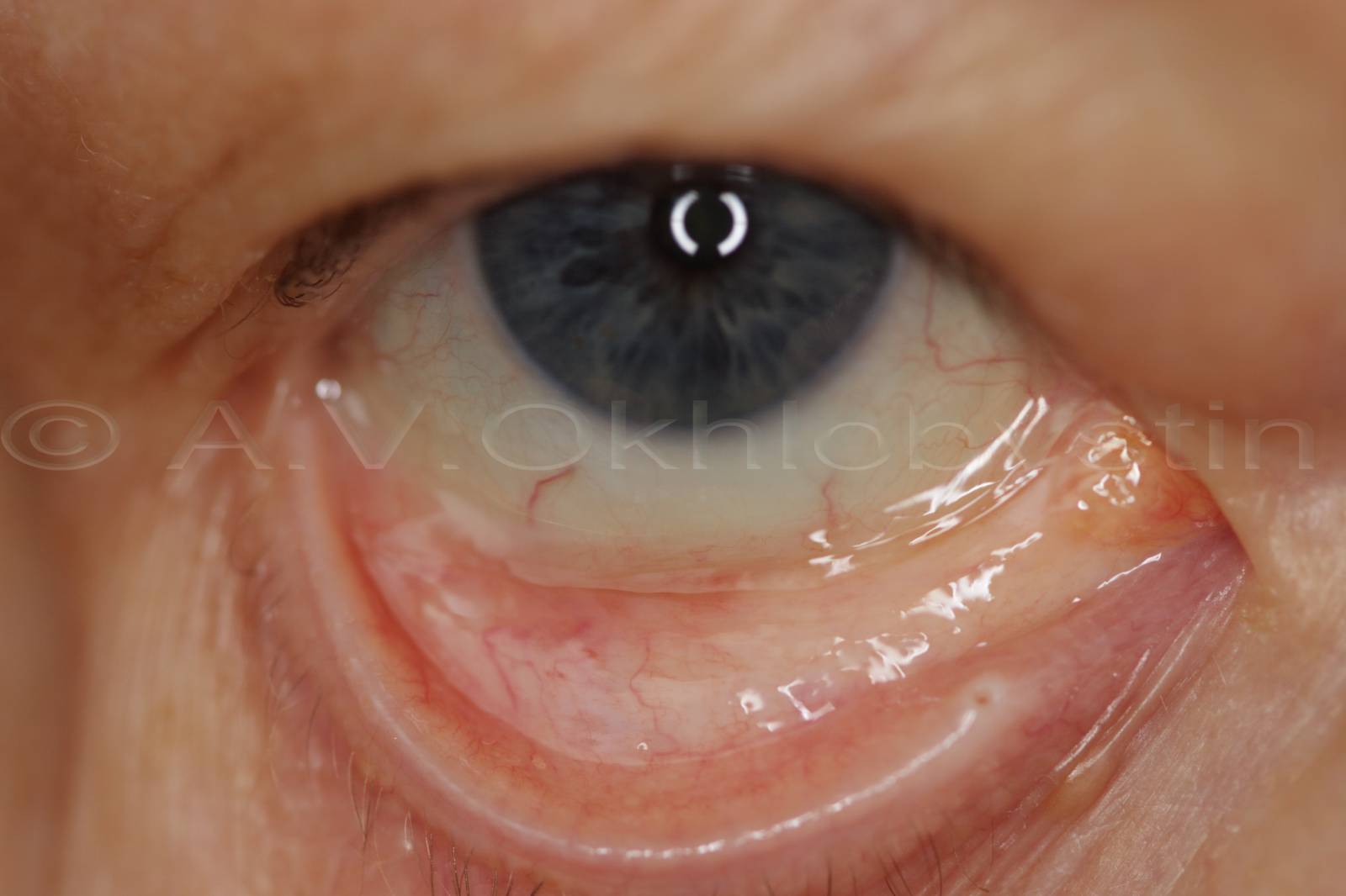
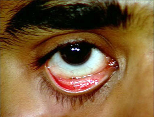
redness = max(0, red - (blue + green) / 2);
I want to identify redness in the image and then compare that value with the redness in another image. I am quite new to Matlab and don't have image processing knowledge. However, I have been trying some random techniques to do this. Till now, I have used histograms of RGB channels of individual images and have also compared average numeric values of RGB channels in individual images. Unfortunately, I see almost similar results in both cases and cannot identify difference between less red and more red image.
I randomly tried working with grayscale histograms as well but found it to be useless.
P.S. I searched on this forum and tried to find a similar problem but i did not find anything that could help me. What I need is: a. Which technique could be used to check redness in images? b. How Matlab can me help there?
%-------------------------------------------
%For histograms of all 3 RGB channels in an image

i = imread('<Path>\a7.png');
imgr = i(:,:,1);
imgg = i(:,:,2);
imgb = i(:,:,3);
histr = hist(imgr(:), bins);
histg = hist(imgg(:), bins);
histb = hist(imgb(:), bins);
hfinal = [histr(:); histg(:); histb(:)];
plot(bins, histr);


%-------------------------------------------
%To compare mean values of R channels of all images

clear all;
%read all images in a sequence
flist=dir('<Path>\*.png');

for p = 1:length(flist)
    for q = 1 : 3
    fread = strcat('<Path>\',flist(p).name);
    im = imread(fread);
    meanim(p,q) = mean2(im(:,:,q));
    end
end

%disp(meanim);
rm = meanim(:,1);
frm = sum(rm(:));
gm = meanim(:,2);
fgm = sum(gm(:));
bm = meanim(:,3);
fbm = sum(bm(:));

figure();
set(0,'DefaultAxesColorOrder',[1 0 0;0 1 0;0 0 1]);
pall = [rm(:), gm(:), bm(:)];
plot(pall);
title('Mean values of R, G and B in 12 images');
leg1 = legend('Red','Green','Blue', ...
                'Location','Best');
print (gcf, '-dbmp', 'rgbchannels.bmp')

sm = sum(meanim);
fsum = sum(sm(:));

% disp(fsum);

f2 = figure(2);
set(f2, 'Name','Average Values');
t = uitable('Parent', f2, 'Position', [20 20 520 380]);
set(t, 'ColumnName', {'Average R', 'Average G', 'Average B'});
set(t, 'Data', pall);
print (gcf, '-dbmp', 'rgbtable.bmp') ;

rgbratio = rm ./ fsum;
disp(rgbratio);

f3 = figure(3);
aind = 1:6;
hold on;
subplot(1,2,1);
plot(rgbratio(aind),'r+');
title('Plot of anemic images - having more pallor');

nind = 7:12;
subplot(1,2,2);
plot(rgbratio(nind),'b.');
title('Plot of non anemic images - having less pallor');
hold off;
print (gcf, '-dbmp', 'anemicpics
------------------------------------------------------------------------------------------------------
You can't assume the red channel is the same as the redness of a pixel by itself. A good estimate of redness of a pixel may be achieved by something like this:
redness = max(0, red - (blue + green) / 2);Where red, green and blue are values of different RGB channels in the image. Once you calculated this value for an image, you can estimate the redness of the image by some approaches like averaging or histograms.
| Using a Gray-Level Co-Occurrence Matrix (GLCM) (0) | 2017.02.03 |
|---|---|
| Embossing filter (0) | 2017.01.13 |
| Taking partial derivatives is easy in Matlab (0) | 2016.12.01 |
| Matlab Image Processing (0) | 2016.12.01 |
| Gabor Filter 이해하기 (0) | 2016.10.17 |


|
| 일 | 월 | 화 | 수 | 목 | 금 | 토 |
|---|---|---|---|---|---|---|
| 1 | 2 | 3 | 4 | |||
| 5 | 6 | 7 | 8 | 9 | 10 | 11 |
| 12 | 13 | 14 | 15 | 16 | 17 | 18 |
| 19 | 20 | 21 | 22 | 23 | 24 | 25 |
| 26 | 27 | 28 | 29 | 30 |


 code.zip