Linear algebra cheat sheet for deep learning
While participating in Jeremy Howard’s excellent deep learning course I realized I was a little rusty on the prerequisites and my fuzziness was impacting my ability to understand concepts like backpropagation. I decided to put together a few wiki pages on these topics to improve my understanding. Here is a prettier version of my linear algebra page.
What is linear algebra?
In the context of deep learning, linear algebra is a mathematical toolbox that offers helpful techniques for manipulating groups of numbers simultaneously. It provides structures like vectors and matrices (spreadsheets) to hold these numbers and new rules for how to add, subtract, multiply, or divide them.
Why is it useful?
It turns complicated problems into simple, intuitive, and efficiently calculated problems. Here is an example of how linear algebra can achieve greater simplicity in code.
# Multiply two arrays
x = [1,2,3]
y = [2,3,4]
product = []
for i in range(len(x)):
    product.append(x[i]*y[i])
# Linear algebra version
x = numpy.array([1,2,3])
y = numpy.array([2,3,4])
x * y
How is it used in deep learning?
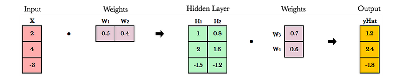
Neural networks store weights in matrices. Linear algebra makes matrix operations fast and easy, especially when training on GPUs. In fact, GPUs were created with vector and matrix operations in mind. Similar to how images can be represented as arrays of pixels, video games generate compelling gaming experiences using enormous, constantly evolving matrices. Instead of processing pixels one-by-one, GPUs manipulate entire matrices of pixels in parallel.
Vectors
Vectors are 1-dimensional arrays of numbers or terms. In geometry, vectors store the magnitude and direction of a potential change to a point in space. The vector [3, -2] for instance says go right 3 and down 2. A vector with more than one dimension is called a matrix.
Vector notation
There are a variety of ways to represent vectors. Here are a few you might come across in your reading.

Vectors in geometry
Vectors typically represent movement from a point. They store both the magnitude and direction of potential changes to a point. The vector [-2,5] says move left 2 units and up 5 units. Source.
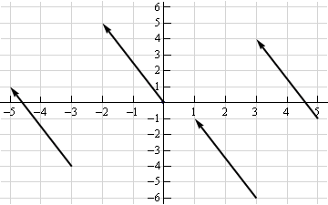
A vector can be applied to any point in space. The vector’s direction equals the slope of the hypotenuse created moving up 5 and left 2. Its magnitude equals the length of the hypotenuse.
Scalar operations
Scalar operations involve a vector and a number. You modify the vector in-place by adding, subtracting, or multiplying the number from all the values in the vector.

Elementwise operations
In elementwise operations like addition, subtraction, and division, values that correspond positionally are combined to produce a new vector. The 1st value in vector A is paired with the 1st value in vector B. The 2nd value is paired with the 2nd, and so on. This means the vectors must have equal dimensions to complete the operation.*

y = np.array([1,2,3])
x = np.array([2,3,4])
y + x = [3, 5, 7]
y - x = [-1, -1, -1]
y / x = [.5, .67, .75]
*In numpy if one of the vectors is of size 1 it can be treated like a scalar and applied to the elements in the larger vector. See below for more details on broadcasting in numpy.
Vector multiplication
There are two types of vector multiplication: Dot product and Hadamard product.
Dot product
The dot product of two vectors is a scalar. Dot product of vectors and matrices (matrix multiplication) is one of the most important operations in deep learning.

y = np.array([1,2,3])
x = np.array([2,3,4])
np.dot(y,x) = 20
Hadamard product
Hadamard Product is elementwise multiplication and it outputs a vector.

y = np.array([1,2,3])
x = np.array([2,3,4])
y * x = [2, 6, 12]
Vector fields
A vector field shows how far the point (x,y) would hypothetically move if we applied a vector function to it like addition or multiplication. Given a point in space, a vector field shows the power and direction of our proposed change at a variety of points in a graph.
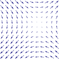
This vector field is an interesting one since it moves in different directions depending the starting point. The reason is that the vector behind this field stores terms like 2x or x² instead of scalar values like -2 and 5. For each point on the graph, we plug the x-coordinate into 2x or x² and draw an arrow from the starting point to the new location. Vector fields are extremely useful for visualizing machine learning techniques like Gradient Descent.
Matrices
A matrix is a rectangular grid of numbers or terms (like an Excel spreadsheet) with special rules for addition, subtraction, and multiplication.
Matrix dimensions
We describe the dimensions of a matrix in terms of rows by columns.
a = np.array([
 [1,2,3],
 [4,5,6]
])
a.shape == (2,3)
b = np.array([
 [1,2,3]
])
b.shape == (1,3)
Matrix scalar operations
Scalar operations with matrices work the same way as they do for vectors. Simply apply the scalar to every element in the matrix — add, subtract, divide, multiply, etc.

a = np.array(
[[1,2],
 [3,4]])
a + 1
[[2,3],
 [4,5]]
Matrix elementwise operations
In order to add, subtract, or divide two matrices they must have equal dimensions.* We combine corresponding values in an elementwise fashion to produce a new matrix.

a = np.array([
 [1,2],
 [3,4]
])
b = np.array([
 [1,2],
 [3,4]
])
a + b
[[2, 4],
 [6, 8]]
a — b
[[0, 0],
 [0, 0]]
Numpy broadcasting*
I can’t escape talking about this, since it’s incredibly relevant in practice. In numpy the dimension requirements for elementwise operations are relaxed via a mechanism called broadcasting. Two matrices are compatible if the corresponding dimensions in each matrix (rows vs rows, columns vs columns) meet the following requirements:
- The dimensions are equal, or
- One dimension is of size 1
a = np.array([
 [1],
 [2]
])
b = np.array([
 [3,4],
 [5,6]
])
c = np.array([
 [1,2]
])
# Same no. of rows
# Different no. of columns
# but a has one column so this works
a * b
[[ 3, 4],
 [10, 12]]
# Same no. of columns
# Different no. of rows
# but c has one row so this works
b * c
[[ 3, 8],
 [5, 12]]
# Different no. of columns
# Different no. of rows
# but both a and c meet the
# size 1 requirement rule
a + c
[[2, 3],
 [3, 4]]
Things get weirder in higher dimensions — 3D, 4D, but for now we won’t worry about that. It’s less common in deep learning.
Matrix Hadamard product
Hadamard product of matrices is an elementwise operation, just like vectors. Values that correspond positionally are multiplied to product a new matrix.

a = np.array(
[[2,3],
 [2,3]])
b = np.array(
[[3,4],
 [5,6]])
# Uses python's multiply operator
a * b
[[ 6, 12],
 [10, 18]]
In numpy you can take the Hadamard product of a matrix and vector as long as their dimensions meet the requirements of broadcasting.

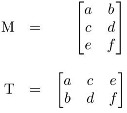
Matrix transpose
Neural networks frequently process weights and inputs of different sizes where the dimensions do not meet the requirements of matrix multiplication. Matrix transpose provides a way to “rotate” one of the matrices so that the operation complies with multiplication requirements and can continue. There are two steps to transpose a matrix:
- Rotate the matrix right 90°
- Reverse the order of elements in each row (e.g. [a b c] becomes [c b a])
As an example, transpose matrix M into T:
a = np.array([
   [1, 2],
   [3, 4]])
a.T
[[1, 3],
 [2, 4]]
Matrix multiplication
Matrix multiplication specifies a set of rules for multiplying matrices together to produce a new matrix.
Rules
Not all matrices are eligible for multiplication. In addition, there is a requirement on the dimensions of the resulting matrix output. Source.
- The number of columns of the 1st matrix must equal the number of rows of the 2nd
- The product of an M x N matrix and an N x K matrix is an M x K matrix. The new matrix takes the rows of the 1st and columns of the 2nd
Steps
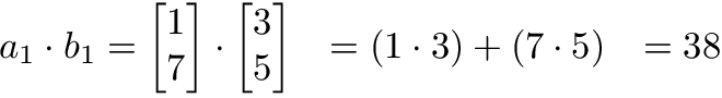
Matrix multiplication relies on dot product to multiply various combinations of rows and columns. In the image below, taken from Khan Academy’s excellent linear algebra course, each entry in Matrix C is the dot product of a row in matrix A and a column in matrix B.
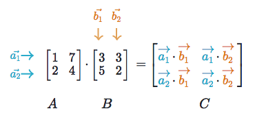
The operation a1 · b1 means we take the dot product of the 1st row in matrix A (1, 7) and the 1st column in matrix B (3, 5).
Here’s another way to look at it:

Why does matrix multiplication work this way?
It’s useful. There is no mathematical law behind why it works this way. Mathematicians developed it because it streamlines previously tedious calculations. It’s an arbitrary human construct, but one that’s extremely useful.
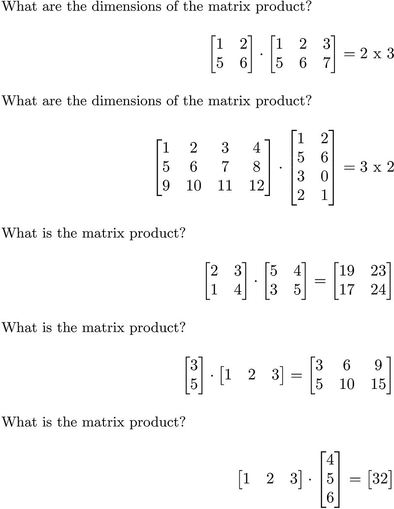
Test yourself with these examples
Matrix multiplication with numpy
Numpy uses the function np.dot(A,B) for both vector and matrix multiplication. It has some other interesting features and gotchas so I encourage you to read the documentation here before use.
a = np.array([
 [1, 2]
 ])
a.shape == (1,2)
b = np.array([
 [3, 4],
 [5, 6]
 ])
b.shape == (2,2)
# Multiply
mm = np.dot(a,b)
mm == [13, 16]
mm.shape == (1,2)
Tutorials
Khan Academy Linear Algebra
Deep Learning Book Math Section
Andrew Ng’s Course Notes
Explanation of Linear Algebra
Explanation of Matrices
Intro To Linear Algebra
Please hit the ♥ button below if you enjoyed reading. Also feel free to suggest new linear algebra concepts I should add to this post!
'Deep Learning > algorithm' 카테고리의 다른 글
| Faster R-CNN 한글 설명 (0) | 2017.03.26 |
|---|---|
| GAN 그리고 Unsupervised Learning (0) | 2017.03.22 |
| 5 algorithms to train a neural network (0) | 2017.03.08 |
| Understanding, generalisation, and transfer learning in deep neural networks (0) | 2017.02.28 |
| Linear Regression / Bias-Variance Decomposition (0) | 2017.01.18 |


