Probabilistic Graphical Models Tutorial — Part 2 – Stats and Bots
https://blog.statsbot.co/probabilistic-graphical-models-tutorial-d855ba0107d1


Homepage
Stats and Bots
Get started
HOMEDATA SCIENCEANALYTICSSTARTUPSBOTSDESIGNSUBSCRIBE TRY STATSBOT FREE
Go to the profile of Prasoon Goyal
Prasoon Goyal
PhD candidate at UT Austin. For more content on machine learning by me, check my Quora profile (https://www.quora.com/profile/Prasoon-Goyal).
Nov 23
Probabilistic Graphical Models Tutorial — Part 2
Parameter estimation and inference algorithms

In the previous part of this probabilistic graphical models tutorial for the Statsbot team, we looked at the two types of graphical models, namely Bayesian networks and Markov networks. We also explored the problem setting, conditional independences, and an application to the Monty Hall problem. In this post, we will cover parameter estimation and inference, and look at another application.

Parameter Estimation
Bayesian networks
Estimating the numbers in the CPD tables of a Bayesian network simply amounts to counting how many times that event occurred in our training data. That is, to estimate p(SAT=s1 | Intelligence = i1), we simply count the fraction of data points where SAT=s1 and Intelligence = i1, out of the total data points where Intelligence = i1. While this approach may appear ad hoc, it turns out that the parameters so obtained maximize the likelihood of the observed data.
Markov networks
For Markov networks, unfortunately, the above counting approach does not have a statistical justification (and will therefore lead to suboptimal parameters). So, we need to use more sophisticated techniques. The basic idea behind most of these techniques is gradient descent — we define parameters that describe the probability distribution, and then use gradient descent to find values for these parameters that maximize the likelihood of the observed data.
Finally, now that we have the parameters of our model, we want to use them on new data, to perform inference!
Inference
The bulk of the literature in probabilistic graphical models focuses on inference. The reasons are two-fold:
Inference is why we came up with this entire framework — being able to make predictions from what we already know.
Inference is computationally hard! In some specific kinds of graphs, we can perform inference fairly efficiently, but on general graphs, it is intractable. So we need to use approximate algorithms that trade off accuracy for efficiency.
There are several questions we can answer with inference:
Marginal inference: Finding the probability distribution of a specific variable. For instance, given a graph with variables A, B, C, and D, where A takes values 1, 2, and 3, find p(A=1), p(A=2) and p(A=3).
Posterior inference: Given some observed variables v_E (E for evidence) that take values e, finding the posterior distribution p(v_H | v_E=e) for some hidden variables v_H.
Maximum-a-posteriori (MAP) inference: Given some observed variables v_E that take values e, finding the setting of other variables v_H that have the highest probability.
Answers to these questions may be useful by themselves, or may need to be used as part of larger tasks.
In what follows, we are going to look at some of the popular algorithms for answering these questions, both exact and approximate. All these algorithms are applicable on both Bayesian networks and Markov networks.
Variable Elimination
Using the definition of conditional probability, we can write the posterior distribution as:

Let’s see how we can compute the numerator and the denominator above, using a simple example. Consider a network with three variables, and the joint distribution defined as follows:

Let’s say we want to compute p(A | B=1). Note that this means that we want to compute the values p(A=0 | B=1)and p(A=1 | B=1), which should sum to one. Using the above equation, we can write

The numerator is the probability that A = 0 and B = 1. We don’t care about the values of C. So we would sum over all the values of C. (This comes from basic probability — p(A=0, B=1, C=0) and p(A=0, B=1, C=1) are mutually exclusive events, so their union p(A = 0, B=1) is just the sum of the individual probabilities.)
So we add rows 3 and 4 to get p(A=0, B=1) = 0.15. Similarly, adding rows 7 and 8 gives usp(A=1, B=1) = 0.40. Also, we can compute the denominator by summing over all rows that contain B=1, that is, rows 3, 4, 7, and 8, to get p(B=1) = 0.55. This gives us the following:
p(A = 0 | B = 1) = 0.15 / 0.55 = 0.27
p(A = 1 | B = 1) = 0.40 / 0.55 = 0.73
If you look at the above computation closely, you would notice that we did some repeated computations — adding rows 3 & 4, and 7 & 8 twice. A more efficient way to compute p(B=1)would have been to simply add the values p(A=0, B=1) and p(A=1, B=1). This is the basic idea of variable elimination.
In general, when you have a lot of variables, not only can you use the values of the numerator to compute the denominator, but the numerator by itself will contain repeated computations, if evaluated naively. You can use dynamic programming to use precomputed values efficiently.
Because we are summing over one variable at a time, thereby eliminating it, the process of summing out multiple variables amounts to eliminating these variables one at a time. Hence, the name “variable elimination.”
It is straightforward to extend the above process to solve the marginal inference or MAP inference problems as well. Similarly, it is easy to generalize the above idea to apply it to Markov networks too.
The time complexity of variable elimination depends on the graph structure, and the order in which you eliminate the variables. In the worst case, it has exponential time complexity.
Belief Propagation
The VE algorithm that we just saw gives us only one final distribution. Suppose we want to find the marginal distributions for all variables. Instead of running variable elimination multiple times, we can do something smarter.
Suppose you have a graph structure. To compute a marginal, you need to sum the joint distribution over all other variables, which amounts to aggregating information from the entire graph. Here’s an alternate way of aggregating information from the entire graph — each node looks at its neighbors, and approximates the distribution of variables locally.
Then, every pair of neighboring nodes send “messages” to each other where the messages contain the local distributions. Now, every node looks at the messages it receives, and aggregates them to update its probability distributions of variables.

In the figure above, C aggregates information from its neighbors A and B, and sends a message to D. Then, D aggregates this message with the information from E and F.
The advantage of this approach is that if you save the messages that you are sending at every node, one forward pass of messages followed by one backward pass gives all nodes information about all other nodes. That information can then be used to compute all the marginals, which was not possible in variable elimination.
If the graph does not contain cycles, then this process converges after a forward and a backward pass. If the graph contains cycles, then this process may or may not converge, but it can often be used to get an approximate answer.
Approximate inference
Because exact inference may be prohibitively time consuming for large graphical models, numerous approximate inference algorithms have been developed for graphical models, most of which fall into one of the following two categories:
Sampling-based
These algorithms estimate the desired probability using sampling. As a simple example, consider the following scenario — given a coin, how you would determine the probability of getting heads when the coin is tossed? The simplest thing is to flip the coin, say, 100 times, and find out the fraction of tosses in which you get heads.
This is a sampling-based algorithm to estimate the probability of heads. For more complex questions in probabilistic graphical models, you can use a similar procedure. Sampling-based algorithms can further be divided into two classes. In the first one, the samples are independent of each other, as in the coin toss example above. These algorithms are called Monte Carlo methods.
For problems with many variables, generating good quality independent samples is difficult, and therefore, we generate dependent samples, that is, each new sample is random, but close to the last sample. Such algorithms are called Markov Chain Monte Carlo (MCMC) methods, because the samples form a “Markov chain.” Once we have the samples, we can use them to answer various inference questions.
Variational methods
Instead of using sampling, variational methods try to approximate the required distribution analytically. Suppose you write out the expression for computing the distribution of interest — marginal probability distribution or posterior probability distribution.
Often, these expressions have summations or integrals in them that are computationally expensive to evaluate exactly. A good way to approximate these expressions is to then solve for an alternate expression, and somehow ensure that this alternate expression is close to the original expression. This is the basic idea behind variational methods.
When we are trying to estimate a complex probability distribution p_complex, we define a separate set of probability distributions P_simple, which are easier to work with, and then find the probability distribution p_approx from P_simple that is closest to p_complex.
Application: Image denoising
Let us now use some of the ideas we just discussed on a real problem. Let’s say you have the following image:

Now suppose that it got corrupted by random noise, so that your noisy image looks as follows:

The goal is to recover the original image. Let’s see how we can use probabilistic graphical models to do this.
The first step is to think about what our observed and unobserved variables are, and how we can connect them to form a graph. Let us define each pixel in the noisy image as an observed random variable, and each pixel in the ground truth image as an unobserved variable. So, if the image is M x N, then there are MN observed variables and MN unobserved variables. Let us denote observed variables as X_ij and unobserved variables as Y_ij. Each variable takes values +1 and -1 (corresponding to black and white pixels, respectively). Given the observed variables, we want to find the most likely values of the unobserved variables. This corresponds to MAP inference.
Now, let us use some domain knowledge to build the graph structure. Clearly, the observed variable at position (i, j) in the noisy image depends on the unobserved variable at position (i, j) in the ground truth image. This is because most of the time, they are identical.
What more can we say? For ground truth images, the neighboring pixels usually have the same values — this is not true at the boundaries of color change, but inside a single-colored region, this property holds. Therefore, we connect Y_ij and Y_kl if they are neighboring pixels.
So, our graph structure looks as follows:

Here, the white nodes denote the unobserved variables Y_ij and the grey nodes denote observed variables X_ij. Each X_ij is connected to the corresponding Y_ij, and each Y_ij is connected to its neighbors.
Note that this is a Markov network, because there is no cause-effect relation between pixels of an image, and therefore, defining directions of arrows in Bayesian networks is unnatural here.
Our MAP inference problem can be mathematically written as follows:

Here, we used some standard simplification techniques common in maximum log likelihood computation. We will use X and Y(without subscripts) to denote the collection of all X_ij and Y_ij values, respectively.
Now, we need to define our joint distribution P(X, Y) based on our graph structure. Let’s assume that P(X, Y) consists of two kinds of factors — ϕ(X_ij, Y_ij) and ϕ(Y_ij,Y_kl), corresponding to the two kinds of edges in our graph. Next, we define the factors as follows:
ϕ(X_ij, Y_ij) = exp(w_e X_ij Y_ij), where w_e is a parameter greater than zero. This factor takes large values when X_ij and Y_ij are identical, and takes small values when X_ij and Y_ij are different.
ϕ(Y_ij, Y_kl) = exp(w_s Y_ij Y_kl), where w_s is a parameter greater than zero, as before. This factor favors identical values of Y_ij and Y_kl.
Therefore, our joint distribution is given by:

where (i, j) and (k, l) in the second product are adjacent pixels, and Z is a normalization constant.
Plugging this into our MAP inference equation gives:

Note that we have dropped the term containing Zsince it does not affect the solution.
The values of w_e and w_s are obtained using parameter estimation techniques from pairs of ground truth and noisy images. This process is fairly mathematically involved (although, at the end of the day, it is just gradient descent on a complicated function), and therefore, we shall not delve into it here. We will assume that we have obtained the following values of these parameters — w_e = 8 and w_s = 10.
The main focus of this example will be inference. Given these parameters, we want to solve the MAP inference problem above. We can use a variant of belief propagation to do this, but it turns out that there is a much simpler algorithm called Iterated conditional modes (ICM) for graphs with this specific structure.
The basic idea is that at each step, you choose one node, Y_ij, look at the value of the MAP inference expression for both Y_ij = -1 and Y_ij = 1, and pick the one with the higher value. Repeating this process for a fixed number of iterations or until convergence usually works reasonably well.
You can use this Python code to do this for our model.
This is the denoised image returned by the algorithm:

Pretty good, isn’t it? Of course, you can use more fancy techniques, both within graphical models, and outside, to generate something better, but the takeaway from this example is that a simple Markov network with a simple inference algorithm already gives you reasonably good results.
Quantitatively, the noisy image has about 10% of the pixels that are different from the original image, while the denoised image produced by our algorithm has about 0.6% of the pixels that are different from the original image.
It is important to note that the graph that we used is fairly large — the image size is about 440 x 300, so the total number of nodes is close to 264,000. Therefore, exact inference in such models is essentially infeasible, and what we get out of most algorithms, including ICM, is a local optimum.
Let’s recap
In this section, let us briefly review the key concepts we covered in this two-part series:
Graphical models: A graphical model consists of a graph structure where nodes represent random variables and edges represent dependencies between variables.
Bayesian networks: These are directed graphical models, with a conditional probability distribution table associated with each node.
Markov networks: These are undirected graphical models, with a potential function associated with each clique.
Conditional independences: Based on how the nodes in the graph are connected, we can write conditional independence statements of the form “X is independent of Y given Z.”
Parameter estimation: Given some data and the graph structure, we want to fill the CPD tables or compute the potential functions.
Inference: Given a graphical model, we want to answer questions about unobserved variables. These questions are usually one of the following — Marginal inference, posterior inference, and MAP inference.
Inference on general graphical models is computationally intractable. We can divide inference algorithms into two broad categories — exact and approximate. Variable elimination and belief propagation in acyclic graphs are examples of exact inference algorithms. Approximate inference algorithms are necessary for large-scale graphs, and usually fall into sampling-based methods or variational methods.
Conclusions
We looked at some of the core ideas in probabilistic graphical models in this two-part tutorial. As you should be able to appreciate at this point, graphical models provide an interpretable way to model many real-world tasks, where there are dependencies. Using graphical models gives us a way to work on such tasks in a principled manner.
Before we close, it is important to point out that this tutorial, by no means, is complete — many details have been skipped to keep the content intuitive and simple. The standard textbook on probabilistic graphical models is over a thousand pages! This tutorial is meant to serve as a starting point, to get you interested in the field, so that you can look up more rigorous resources.
Here are some additional resources that you can use to dig deeper into the field:
Graphical Models in a Nutshell
Graphical Models textbook
You should also be able to find a few chapters on graphical models in standard machine learning textbooks.

YOU’D ALSO LIKE:
Probabilistic Graphical Models Tutorial — Part 1

Basic terminology and the problem setting
blog.statsbot.co
Machine Learning Algorithms: Which One to Choose for Your Problem

Intuition of using different kinds of algorithms in different tasks
blog.statsbot.co
Neural networks for beginners: popular types and applications

An introduction to neural networks learning
blog.statsbot.co
Machine LearningData ScienceAlgorithmsBayesian StatisticsMarkov Chains
One clap, two clap, three clap, forty?
By clapping more or less, you can signal to us which stories really stand out.


265

Follow
Go to the profile of Prasoon Goyal
Prasoon Goyal
PhD candidate at UT Austin. For more content on machine learning by me, check my Quora profile (https://www.quora.com/profile/Prasoon-Goyal).
Follow
Stats and Bots
Stats and Bots
Data stories on machine learning and analytics. From Statsbot’s makers.
More from Stats and Bots
Neural networks for beginners: popular types and applications
Go to the profile of Jay Shah
Jay Shah

287

Also tagged Markov Chains
Implementing Markov Chain in Swift. Generating Texts.
Go to the profile of Swift The Sorrow
Swift The Sorrow

41

More on Algorithms from Stats and Bots
Data Structures Related to Machine Learning Algorithms
Go to the profile of Peter Mills
Peter Mills

275
Posted by uniqueone
,

MNIST Kaggle submission with CNN Keras Swish activation
https://medium.com/@shahariarrabby/mnist-kaggle-submission-with-cnn-keras-switch-activation-62108f9463df
Posted by uniqueone
,
https://blog.acolyer.org/


Posted by uniqueone
,

Faster R-CNN
https://curt-park.github.io/2017-03-17/faster-rcnn/
Posted by uniqueone
,

T-Robotics: GAN 그리고 Unsupervised Learning
http://t-robotics.blogspot.kr/2017/03/gan-unsupervised-learning.html?m=1


T-Robotics
2017년 3월 8일 수요일
GAN 그리고 Unsupervised Learning
이 글은 테크M에 기고한 글을 백업한 글입니다.

머신러닝 분야 세계 최고 학회중 하나인 NIPS에서 중국 바이두의  인공지능연구소장, 앤드류 응은 최근 머신러닝 트렌드를 이렇게 진단했다.
“이미지 인식, 음성 인식 등 이제까지 구글 같은 거대기업에 돈을 벌어 준 딥러닝 기술은 컨볼루셔널 신경망(CNN)이나 재귀신경망(RNN) 같은 지도학습 기술이었습니다. 하지만 올해 나온 많은 논문들이 보여주는 것처럼, 미래의 딥러닝을 이끌 기술은 생성적 적대신경망(GAN)과 같은 비지도 학습이 그 주인공이 될 것입니다.”
이러한 견해를 보이는 것은 응 교수만이 아니다. 많은 딥러닝 연구자들이 꾸준히 제기하고 있는 이야기이기도 하다. 지도학습은 많은 데이터의 지원을 받는 환경에서는  좋은 성능을 내지만, 그것은 미래 인공지능이 다뤄야 할 ‘경험의 진정한 이해’와는 큰 차이가 있다는 것이다.
“내가 다시 창조할 수 없는 것은 내가 이해한 것이 아니다.”      (물리학자 리처드 파인만)
많은 인공지능 전문가들이 미래를 이끌 것으로 전망하는 비지도 학습은 생성 모델(generative model)과 긴밀히 연결돼 있다. 기존의 CNN과 RNN은 이미지를 구별하고 음성을 인식하지만 이미지나 음성을 만들지는 못했다.
하지만 미래의 생성 모델을 활용하면 직접 이미지와 음성을 만들어낼 수 있다. 단순히 알아보기만 하던 것에서 한 발 나아가 직접 그림을 그릴 수 있는 것으로의 진보, 그 중심에는 2014년 처음 발표된 GAN이 있다.
GAN의 개발자이자 오픈AI의 수석연구원인 이안 굿 펠로우. 그는 캐나다 몬트리올대학 벤지오 교수의 애제자이기도 하다.

지도 학습과 생성 모델

그럼 우선 지도학습(supervised learning)과 비지도 학습(unsupervised learning)의 차이를 알아보자.
지금까지 머신러닝의 주류를 이뤘던  지도학습은 데이터와 라벨(이름)의 짝을 집중 학습하는 방법이었다. 컴퓨터를 아이라고 가정하면, 여러 개의 사물을 보여주면서  ‘이것은 개’, ‘이것은 고양이’, ‘이것은 식탁’ 하고 사물 X와 이름 Y의 쌍을 지속적으로 학습시키는 것이다.
이렇게 수많은 (X, Y)의 함수를 알게 되면 전혀 알지 못하는 미지의 사물 X에 대해서도 적절한 예측 Y를 내놓을 수 있게 된다. 구글과 페이스북 등에서 사용하는 얼굴인식이나 사물인식, 음성인식 모두 이러한 지도학습 방법을 이용한 기술들이었다.

하지만 이 방법에는 한계가 있다. 누군가 일일이 각 사물의 ‘정답(label)’을 알려 줘야 만 학습이 가능하기 때문이다. 페이스북에 인물사진을 올리면 사진에 있는 얼굴이 누구인지 이용자들이 직접 써 넣도록 유도하는 데, 이러한 라벨링은 결국 특정 인물을 인식하게 하는 큰 원동력이 된다. 반대로 얘기하자면, 이러한 라벨링이 없다면 지식을 얻을 수 없고 학습도 할 수 없다는 게 현재 지도학습의 한계다.

하지만 아이가 사물들을 알아가는 방식을 생각해보자.  아이들은 꼭 누가 일일이 그 사물이 무엇인지 알려줘야만 사물에 대해 배우는 것은 아니다. 다양한 모양의 장난감 블록을 주고 가지고 놀게 하면, 아이는 스스로 네모와 세모, 동그라미의 차이를 터득하게 된다.
궁극적인 인공지능을 구현하려면 이렇게 누군가 정답을 가르쳐주지 않더라도 인공지능 스스로 사물의 특성을 파악할 수 있는 능력이 있어야 한다. 이렇게 라벨 없이 데이터 그 자체에서 지식을 얻는 방법을 비지도 학습이라고 한다.

비지도 학습이 미래 기술로서 주목 받는 이유는, 세상에는 (라벨링이 된 데이터의 양에 비해) 엄청나게 많은 라벨 없는 데이터들이 존재하기 때문이다. 사진만 해도 그렇다. 우리는 수많은 사진을 찍지만 사진 속 얼굴이 누구이고 이 사물이 무엇인지 라벨링을 해주는 경우는 극소수에 불과하다.
지금까지 지도학습 기반의 딥러닝 기술이 이렇게 발전할 수 있었던 것도 이미지넷이나 CIFAR 같은 라벨링이 잘 돼 있는 공공데이터의 존재 덕분이었다. 그런데 이 딥러닝의 혜택을 실제 세계에 옮겨오려면 (세상에 존재하는 수많은 라벨 없는 데이터들을 이용하려면) 비지도 학습의 발전이 없으면 불가능하다.

그 미래 기술의 물꼬를 튼 기술이 바로 GAN(Generative Adversarial Network) 이었다. 이전에도 제한 볼츠만 머신(RBM)이나 자동 엔코더 같은 비지도 학습 방법이 있기는 했다. 하지만 이 방법은 지도학습을 위한 사전 처리의 용도 외에는 활용하기가 쉽지 않았다.
하지만  ‘지도학습 같은 비지도 학습’인  GAN은 놀라운 성능과 함께 지도학습 못지 않은 활용도를 보여 머신러닝 연구의  중심에 섰다. 페이스북의 얀 르쿤이 “지난 10년간 있었던 머신러닝 연구 중 가장 재미있는 아이디어”라고 평했던 GAN은 대체 어떤 기술일까?

모조품과의 경쟁을 통해 배운다

GAN은 그동안 좋은 성과를 냈던 지도학습의 훈련방법을 비지도 학습에도 적용했다. ‘정답’에 대한 정보가 없는 상황에서 어떻게 지도학습의 방법을 차용했을까?

먼저 최대한 진짜 같은 샘플을 만드는 것을 목표로 한다. (앞의 ‘이해한다는 것은 새로 창조할 수 있다는 말이다’란 명언을 기억하자.) 비지도 학습법은 실제 데이터로 대강의 함수를 표현하고 이를 다시 적당히 일반화 해 새 데이터를 만들 수는 있었다.
예를 들어 10살과 20살의 얼굴 모습이 있다면, 이 변화과정을 적절히 모델링 해 15살의 얼굴을 만드는 것이다. 하지만 이 방법은 확률모델에 많은 가정을 해야 하고 다양한 데이터들이 평균점을 향해 섞여 결과적으로는 ‘뭉개진(blurry)’ 이미지를 만들어낸다는 단점을 가지고 있었다.

하지만 GAN은 ‘만드는 사람(generator)’과 ‘구별하는 사람(discriminator)’이 서로 경쟁하는 게임으로 바꿔 모델 학습을 시도했다. 비유를 하자면 화폐위조범(=generator)은 최대한 진짜 같은 화폐를 만들기 위해 노력하고, 감별사(=discriminator)는 진짜와 가짜 화폐를 구분하기 위해 노력함으로써 서로의 발전을 꾀하는 것이다(라이벌은 서로를 발전시킨다!).

GAN은 생성자(모조품 제작자)와 구별자(진품 감별사) 사이의 경쟁적 발전을 통해 좀 더 진짜에 가까운 샘플을 만든다.
여기서 구별하는 사람은 기존 지도학습 방법의 ‘인식 기술’과 같은 기술을 사용한다. 따라서 구별하는 사람을 속이려면 매우 좋은 품질의 위조품을 만들어야 하고, 결과적으로 스스로가 뛰어난 만드는 사람이 되는 학습을 하게 되는 것이다.
‘학습’을 ‘경쟁게임’으로 바꾼 GAN의 아이디어는 기존 비지도 학습의 난제를 피하면서도 지도학습의 기술들을 활용할 수 있는 매우 똑똑한 아이디어라 할 수 있다.

이 결과, GAN은 기존의 생성모델처럼 뭉개지지 않는, 더 생생한 이미지들을 만들어 낼 수 있었다. 뿐만 아니라, 사용자가 입력한 조건에 가장 가까운 샘플을 생성할 수도 있다. 사용자가 대충 스케치를 하면 진짜 같은 그림을 생성해주는 이미지 편집의 기능도 구현할 수 있게 해준 것이다. 또 흐려진 이미지에 대해 ‘진짜 같아지는 학습’을 통해 더욱 선명한 이미지로 복원하는 기능을 제공했고, 위성사진을 지도사진으로 변환하는 등 사진과 사진의 전환(image to image transfer)도 가능하게 해주었다.

GAN을 이용한 이미지 복원(위)과 GAN을 이용한 사진과 사진의 전환 (아래)

DC-GAN을 이용해 생성된 침실 이미지들. 모두 실제 사진들 같아 보이지만 몇몇 사진들은 논리적으로 맞지 않는 침실모습을 갖고 있다.


GAN과 인공지능의 미래

GAN의 등장으로 인해 인공지능은 ‘수동적 인식’에서 벗어나 ‘능동적 행동’을 할 수 있는 인공지능으로 진일보하고 있다. 이안 굿 펠로우가 GAN을 발표한지 채 2년 밖에 되지 않았지만, GAN은 이미지 생성부터 편집, 변환, 복원 등 다양한 어플리케이션에서 그 효용을 보여주고 있다. 2017년에는 이미지 데이터를 넘어 음성이나 자연어 등의 데이터에도 GAN이 적용될 전망이다. 이를 이용하면 음성 생성과 편집, 음성 변환이나 복원 등도 가능하지 않을까 기대해본다.
이론적으로는 ‘학습’에서 ‘경쟁게임’으로 전환하여 푸는 방식이 매우 흥미로운 접근법이었는데, 최적화를 기반으로 한 학습에 치우쳐 있던 머신러닝의 기법들이 ‘경쟁게임’을 활용해 어떠한 방향으로 발전해 나갈지 기대가 크다.

GAN의 가장 큰 약점은 만드는 쪽과 구별하는 쪽을 균형 있게 훈련시키기가 기존의 최적화에 비해 매우 어렵다는 것이다. 게임을 하는 두 사람 간의 실력 차가 크다면 서로의 발전을 기대하기는 어렵다.  GAN의 학습도 이러한 ‘실력 차’에 의한 불균형이 종종 발생해 훈련을 어렵게 하곤 한다.
하지만 현재 이를 피하기 위한 여러 가지 트릭이 제시되고 있으며, 이와 함께 적대적 게임관계의 효율적 수렴을 위한 이론적 연구가 앞으로 많이 진행될 전망이다. 또 아직까지 정적인 데이터인 이미지에만 주로 사용되는 GAN을 음성이나 자연어 등에 확장시키려면 순서(sequence) 데이터를 고려한 알고리즘의 변형이 필요할 것으로 보인다.

인공지능은 GAN을 통해 수동적 존재에서 능동적 존재로의 첫 발을 내디뎠다. 비록 아직은 데이터로 재미있는 변화들을 만들어내는 수준에 불과하지만, 이들을 통해 스스로 새로운 지식을 쌓고 학습하는데(self-learning)까지 얼마가 더 걸릴지는 모르는 일이다.
인간이 데이터를 제공하는 것에서 벗어나 스스로 환경과 상호작용하며 경험을 축적하는 능동적 인공지능을 개발하려면 지식을 탐닉하는 에이전트가 필요하다. 이를 위해선 현재 게임에 많이 적용되고 있는 강화학습(reinforcement learning)과의 결합이 필요해 보인다.

[facebook] http://facebook.com/trobotics
[rss] http://t-robotics.blogspot.kr/feeds/posts/default


Terry TaeWoong Um [Date] 3/08/2017
공유


웹 버전 보기

 
Powered by Blogger.
Posted by uniqueone
,
https://medium.com/towards-data-science/linear-algebra-cheat-sheet-for-deep-learning-cd67aba4526c#.2dqnqasml


Linear algebra cheat sheet for deep learning

While participating in Jeremy Howard’s excellent deep learning course I realized I was a little rusty on the prerequisites and my fuzziness was impacting my ability to understand concepts like backpropagation. I decided to put together a few wiki pages on these topics to improve my understanding. Here is a prettier version of my linear algebra page.

What is linear algebra?

In the context of deep learning, linear algebra is a mathematical toolbox that offers helpful techniques for manipulating groups of numbers simultaneously. It provides structures like vectors and matrices (spreadsheets) to hold these numbers and new rules for how to add, subtract, multiply, or divide them.

Why is it useful?

It turns complicated problems into simple, intuitive, and efficiently calculated problems. Here is an example of how linear algebra can achieve greater simplicity in code.

# Multiply two arrays 
x = [1,2,3]
y = [2,3,4]
product = []
for i in range(len(x)):
product.append(x[i]*y[i])
# Linear algebra version
x = numpy.array([1,2,3])
y = numpy.array([2,3,4])
x * y

How is it used in deep learning?

Neural networks store weights in matrices. Linear algebra makes matrix operations fast and easy, especially when training on GPUs. In fact, GPUs were created with vector and matrix operations in mind. Similar to how images can be represented as arrays of pixels, video games generate compelling gaming experiences using enormous, constantly evolving matrices. Instead of processing pixels one-by-one, GPUs manipulate entire matrices of pixels in parallel.

Vectors

Vectors are 1-dimensional arrays of numbers or terms. In geometry, vectors store the magnitude and direction of a potential change to a point in space. The vector [3, -2] for instance says go right 3 and down 2. A vector with more than one dimension is called a matrix.

Vector notation

There are a variety of ways to represent vectors. Here are a few you might come across in your reading.

Vectors in geometry

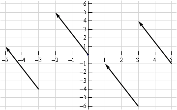
Vectors typically represent movement from a point. They store both the magnitude and direction of potential changes to a point. The vector [-2,5] says move left 2 units and up 5 units. Source.

v = [-2, 5]

A vector can be applied to any point in space. The vector’s direction equals the slope of the hypotenuse created moving up 5 and left 2. Its magnitude equals the length of the hypotenuse.

Scalar operations

Scalar operations involve a vector and a number. You modify the vector in-place by adding, subtracting, or multiplying the number from all the values in the vector.

Scalar addition

Elementwise operations

In elementwise operations like addition, subtraction, and division, values that correspond positionally are combined to produce a new vector. The 1st value in vector A is paired with the 1st value in vector B. The 2nd value is paired with the 2nd, and so on. This means the vectors must have equal dimensions to complete the operation.*

Vector addition
y = np.array([1,2,3])
x = np.array([2,3,4])
y + x = [3, 5, 7]
y - x = [-1, -1, -1]
y / x = [.5, .67, .75]

*In numpy if one of the vectors is of size 1 it can be treated like a scalar and applied to the elements in the larger vector. See below for more details on broadcasting in numpy.

Vector multiplication

There are two types of vector multiplication: Dot product and Hadamard product.

Dot product

The dot product of two vectors is a scalar. Dot product of vectors and matrices (matrix multiplication) is one of the most important operations in deep learning.

y = np.array([1,2,3])
x = np.array([2,3,4])
np.dot(y,x) = 20

Hadamard product

Hadamard Product is elementwise multiplication and it outputs a vector.

y = np.array([1,2,3])
x = np.array([2,3,4])
y * x = [2, 6, 12]

Vector fields

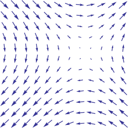
A vector field shows how far the point (x,y) would hypothetically move if we applied a vector function to it like addition or multiplication. Given a point in space, a vector field shows the power and direction of our proposed change at a variety of points in a graph.

Source

This vector field is an interesting one since it moves in different directions depending the starting point. The reason is that the vector behind this field stores terms like 2x or instead of scalar values like -2 and 5. For each point on the graph, we plug the x-coordinate into 2x or and draw an arrow from the starting point to the new location. Vector fields are extremely useful for visualizing machine learning techniques like Gradient Descent.

Matrices

A matrix is a rectangular grid of numbers or terms (like an Excel spreadsheet) with special rules for addition, subtraction, and multiplication.

Matrix dimensions

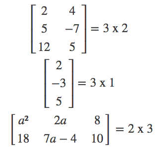
We describe the dimensions of a matrix in terms of rows by columns.

a = np.array([
[1,2,3],
[4,5,6]
])
a.shape == (2,3)
b = np.array([
[1,2,3]
])
b.shape == (1,3)

Matrix scalar operations

Scalar operations with matrices work the same way as they do for vectors. Simply apply the scalar to every element in the matrix — add, subtract, divide, multiply, etc.

Matrix scalar addition
a = np.array(
[[1,2],
[3,4]])
a + 1
[[2,3],
[4,5]]

Matrix elementwise operations

In order to add, subtract, or divide two matrices they must have equal dimensions.* We combine corresponding values in an elementwise fashion to produce a new matrix.

a = np.array([
[1,2],
[3,4]
])
b = np.array([
[1,2],
[3,4]
])
a + b
[[2, 4],
[6, 8]]
a — b
[[0, 0],
[0, 0]]

Numpy broadcasting*

I can’t escape talking about this, since it’s incredibly relevant in practice. In numpy the dimension requirements for elementwise operations are relaxed via a mechanism called broadcasting. Two matrices are compatible if the corresponding dimensions in each matrix (rows vs rows, columns vs columns) meet the following requirements:

  1. The dimensions are equal, or
  2. One dimension is of size 1
a = np.array([
[1],
[2]
])
b = np.array([
[3,4],
[5,6]
])
c = np.array([
[1,2]
])
# Same no. of rows
# Different no. of columns
# but a has one column so this works
a * b
[[ 3, 4],
[10, 12]]
# Same no. of columns
# Different no. of rows
# but c has one row so this works
b * c
[[ 3, 8],
[5, 12]]
# Different no. of columns
# Different no. of rows
# but both a and c meet the
# size 1 requirement rule
a + c
[[2, 3],
[3, 4]]

Things get weirder in higher dimensions — 3D, 4D, but for now we won’t worry about that. It’s less common in deep learning.

Matrix Hadamard product

Hadamard product of matrices is an elementwise operation, just like vectors. Values that correspond positionally are multiplied to product a new matrix.

a = np.array(
[[2,3],
[2,3]])
b = np.array(
[[3,4],
[5,6]])
# Uses python's multiply operator
a * b
[[ 6, 12],
[10, 18]]

In numpy you can take the Hadamard product of a matrix and vector as long as their dimensions meet the requirements of broadcasting.

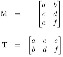
Matrix transpose

Neural networks frequently process weights and inputs of different sizes where the dimensions do not meet the requirements of matrix multiplication. Matrix transpose provides a way to “rotate” one of the matrices so that the operation complies with multiplication requirements and can continue. There are two steps to transpose a matrix:

  1. Rotate the matrix right 90°
  2. Reverse the order of elements in each row (e.g. [a b c] becomes [c b a])

As an example, transpose matrix M into T:

a = np.array([
[1, 2],
[3, 4]])
a.T
[[1, 3],
[2, 4]]

Matrix multiplication

Matrix multiplication specifies a set of rules for multiplying matrices together to produce a new matrix.

Rules

Not all matrices are eligible for multiplication. In addition, there is a requirement on the dimensions of the resulting matrix output. Source.

  1. The number of columns of the 1st matrix must equal the number of rows of the 2nd
  2. The product of an M x N matrix and an N x K matrix is an M x K matrix. The new matrix takes the rows of the 1st and columns of the 2nd

Steps

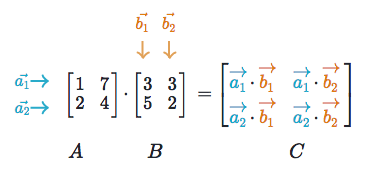
Matrix multiplication relies on dot product to multiply various combinations of rows and columns. In the image below, taken from Khan Academy’s excellent linear algebra course, each entry in Matrix C is the dot product of a row in matrix A and a column in matrix B.

Source

The operation a1 · b1 means we take the dot product of the 1st row in matrix A (1, 7) and the 1st column in matrix B (3, 5).

Here’s another way to look at it:

Why does matrix multiplication work this way?

It’s useful. There is no mathematical law behind why it works this way. Mathematicians developed it because it streamlines previously tedious calculations. It’s an arbitrary human construct, but one that’s extremely useful.

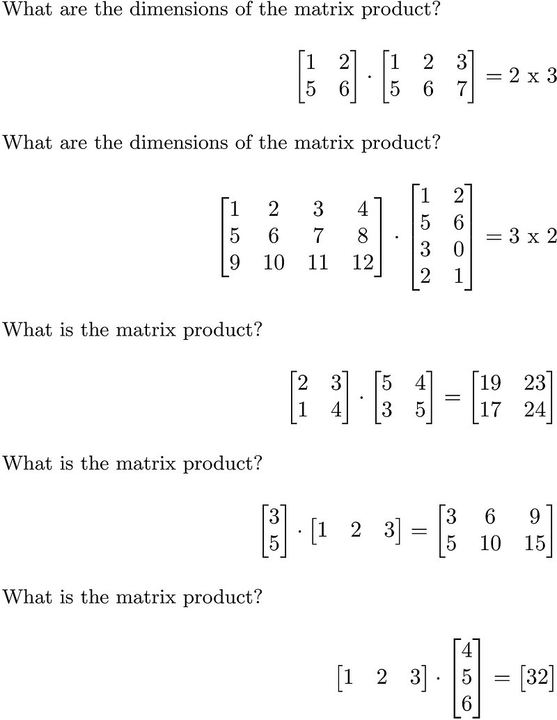
Test yourself with these examples

Matrix multiplication with numpy

Numpy uses the function np.dot(A,B) for both vector and matrix multiplication. It has some other interesting features and gotchas so I encourage you to read the documentation here before use.

a = np.array([
[1, 2]
])
a.shape == (1,2)
b = np.array([
[3, 4],
[5, 6]
])
b.shape == (2,2)
# Multiply
mm = np.dot(a,b)
mm == [13, 16]
mm.shape == (1,2)

Tutorials

Khan Academy Linear Algebra
Deep Learning Book Math Section
Andrew Ng’s Course Notes
Explanation of Linear Algebra
Explanation of Matrices
Intro To Linear Algebra


Please hit the ♥ button below if you enjoyed reading. Also feel free to suggest new linear algebra concepts I should add to this post!

Posted by uniqueone
,

https://www.neuraldesigner.com/blog/5_algorithms_to_train_a_neural_network


5 algorithms to train a neural network

By Alberto Quesada, Artelnics.


algorithm picture

The procedure used to carry out the learning process in a neural network is called the training algorithm. There are many different training algorithms, whith different characteristics and performance.

Problem formulation

The learning problem in neural networks is formulated in terms of the minimization of a loss function, f. This function is in general, composed of an error and a regularization terms. The error term evaluates how a neural network fits the data set. On the other hand, the regularization term is used to prevent overfitting, by controlling the effective complexity of the neural network.

The loss function depends on the adaptative parameters (biases and synaptic weights) in the neural network. We can conveniently group them together into a single n-dimensional weight vector w. The picture below represents the loss function f(w).

Loss function picture


As we can see in the previous picture, the point w* is minima of the loss function. At any point A, we can calculate the first and second derivatives of the loss function. The first derivatives are gropued in the gradient vector, whose elements can be written

if(w) = df/dwi (i = 1,...,n)


Similarly, the second derivatives of the loss function can be grouped in the Hessian matrix,

Hi,jf(w) = d2f/dwi·dwj (i,j = 1,...,n)


The problem of minimizing continuous and differentiable functions of many variables has been widely studied. Many of the conventional approaches to this problem are directly applicable to that of training neural networks.

One-dimensional optimization

Although the loss function depends on many parameters, one-dimensional optimization methods are of great importance here. Indeed, they are are very often used in the training process of a neural network.

Indeed, many training algorithms first compute a training direction d and then a traning rate η that minimizes the loss in that direction, f(η). The next picture illustrates this one-dimensional function.

one-dimensional function picture


The points η1 and η2 define an interval that contains the minimum of f, η*.

In this regard, one-dimensional optimization methods search for the minimum of a given one-dimensional function. Some of the algorithms which are widely used are the golden section method and the Brent's method. Both reduce the bracket of a minumum until the distance between the two outer points in the bracket is less than a defined tolerance.

Multidimensional optimization

The learning problem for neural networks is formulated as searching of a parameter vector w* at which the loss function f takes a minimum value. The necessary condition states that if the neural network is at a minimum of the loss function, then the gradient is the zero vector.

The loss function is, in general, a non linear function of the parameters. As a consequence, it is not possible to find closed training algorithms for the minima. Instead, we consider a search through the parameter space consisting of a succession of steps. At each step, the loss will decrease by adjusting the neural network parameters.

In this way, to train a neural network we start with some parameter vector (often chosen at random). Then, we generate a sequence of parameters, so that the loss function is reduced at each iteration of the algorithm. The change of loss between two steps is called the loss decrement. The training algorithm stops when a specified condition, or stopping criterion, is satisfied.

Now, we are going to describe the most importat training algorithms for neural networks.

Algorithm types


1. Gradient descent

Gradient descent, also known as steepest descent, is the simplest training algorithm. It requires information from the gradient vector, and hence it is a first order method.

Let denote f(wi) = fi and ᐁf(wi) = gi. The method begins at a point w0 and, until a stopping criterion is satisfied, moves from wi to wi+1 in the training direction di = -gi. Therefore, the gradient descent method iterates in the following way:

wi+1 = wi - di·ηi,   i=0,1,...


The parameter η is the training rate. This value can either set to a fixed value or found by one-dimensional optimization along the training direction at each step. An optimal value for the training rate obtained by line minimization at each successive step is generally preferable. However, there are still many software tools that only use a fixed value for the training rate.

The next picture is an activity diagram of the training process with gradient descent. As we can see, the parameter vector is improved in two steps: First, the gradient descent training direction is computed. Second, a suitable training rate is found.

Gradient descent diagram


The gradient descent training algorithm has the severe drawback of requiring many iterations for functions which have long, narrow valley structures. Indeed, the downhill gradient is the direction in which the loss function decreases most rapidly, but this does not necessarily produce the fastest convergence. The following picture illustrates this issue.

Gradient descent picture


Gradient descent is the recommended algorithm when we have very big neural networks, with many thousand parameters. The reason is that this method only stores the gradient vector (size n), and it does not store the Hessian matrix (size n2).

2. Newton's method

The Newton's method is a second order algorithm because it makes use of the Hessian matrix. The objective of this method is to find better training directions by using the second derivatives of the loss function.

Let denote f(wi) = fi, ᐁf(wi) = gi and Hf(wi) = Hi. Consider the quadratic approximation of f at w0 using the Taylor's series expansion

f = f0 + g0 · (w - w0) + 0.5 · (w - w0)2 · H0


H0 is the Hessian matrix of f evaluated at the point w0. By setting g equal to 0 for the minimum of f(w), we obtain the next equation

g = g0 + H0 · (w - w0) = 0


Therefore, starting from a parameter vector w0, Newton's method iterates as follows

wi+1 = wi - Hi-1·gi,   i=0,1,...


The vector Hi-1·gi is known as the Newton's step. Note that this change for the parameters may move towards a maximum rather than a minimum. This occurs if the Hessian matrix is not positive definite. Thus, the function evaluation is not guaranteed to be reduced at each iteration. In order to prevent such troubles, the Newton's method equation usually modified as:

wi+1 = wi - (Hi-1·gi)·ηi,   i=0,1,...


The training rate, η, can either set to a fixed value or found by line minimization. The vector d = Hi-1·gi is now called the Newton's training direction.

The state diagram for the training process with the Newton's method is depicted in the next figure. Here improvement of the parameters is performed by obtaining first the Newton's training direction and then a suitable training rate.

Newton's method diagram


The picture below illustrates the performance of this method. As we can see, the Newton's method requires less steps than gradient descent to find the minimum value of the loss function.

Newton's method graph


However, the Newton's method has the difficulty that the exact evaluation of the Hessian and its inverse are quite expensive in computational terms.


3. Conjugate gradient

The conjugate gradient method can be regarded as something intermediate between gradient descent and Newton's method. It is motivated by the desire to accelerate the typically slow convergence associated with gradient descent. This method also avoids the information requirements associated with the evaluation, storage, and inversion of the Hessian matrix, as required by the Newton's method.

In the conjugate gradient training algorithm, the search is performed along conjugate directions which produces generally faster convergence than gradient descent directions. These training directions are conjugated with respect to the Hessian matrix.

Let denote d the training direction vector. Then, starting with an initial parameter vector w0 and an initial training direction vector d0 = -g0, the conjugate gradient method constructs a sequence of training directions as:

di+1 = gi+1 + di·γi,   i=0,1,...


Here γ is called the conjugate parameter, and there are different ways to calculate it. Two of the most used are due to Fletcher and Reeves and to Polak and Ribiere. For all conjugate gradient algorithms, the training direction is periodically reset to the negative of the gradient.

The parameters are then improved according to the next expression. The training rate, η, is usually found by line minimization.

wi+1 = wi + di·ηi,   i=0,1,...


The picture below depicts an activity diagram for the training process with the conjugate gradient. Here improvement of the parameters is done by first computing the conjugate gradient training direction and then suitable training rate in that direction.

Conjugate gradient diagram


This method has proved to be more effective than gradient descent in training neural networks. Since it does not require the Hessian matrix, conjugate gradient is also recommended when we have very big neural networks.


4. Quasi-Newton method

Application of the Newton's method is computationally expensive, since it requires many operations to evaluate the Hessian matrix and compute its inverse. Alternative approaches, known as quasi-Newton or variable metrix methods, are developed to solve that drawback. These methods, instead of calculating the Hessian directly and then evaluating its inverse, build up an approximation to the inverse Hessian at each iteration of the algorithm. This approximation is computed using only information on the first derivatives of the loss function.

The Hessian matrix is composed of the second partial derivatives of the loss function. The main idea behind the quasi-Newton method is to approximate the inverse Hessian by another matrix G, using only the first partial derivatives of the loss function. Then, the quasi-Newton formula can be expressed as:

wi+1 = wi - (Gi·gi)·ηi,   i=0,1,...


The training rate η can either set to a fixed value or found by line minimization. The inverse Hessian approximation G has different flavours. Two of the most used are the Davidon–Fletcher–Powell formula (DFP) and the Broyden–Fletcher–Goldfarb–Shanno formula (BFGS).

The activity diagram of the quasi-Newton training process is illustrated bellow. Improvement of the parameters is performed by first obtaining the quasi-Newton training direction and then finding a satisfactory training rate.

Quasi newton algorithm diagram


This is the default method to use in most cases: It is faster than gradient descent and conjugate gradient, and the exact Hessian does not need to be computed and inverted.


5. Levenberg-Marquardt algorithm

The Levenberg-Marquardt algorithm, also known as the damped least-squares method, has been designed to work specifically with loss functions which take the form of a sum of squared errors. It works without computing the exact Hessian matrix. Instead, it works with the gradient vector and the Jacobian matrix.

Consider a loss function which can be expressed as a sum of squared errors of the form

f = ∑ ei2,   i=0,...,m


Here m is the number of instances in the data set.


We can define the Jacobian matrix of the loss function as that containing the derivatives of the errors with respect to the parameters,

Ji,jf(w) = dei/dwj (i = 1,...,m & j = 1,...,n)


Where m is the number of instances in the data set and n is the number of parameters in the neural network. Note that the size of the Jacobian matrix is m·n.


The gradient vector of the loss function can be computed as:

ᐁf = 2 JT·e


Here e is the vector of all error terms.


Finally, we can approximate the Hessian matrix with the following expression.

Hf ≈ 2 JT·J + λI


Where λ is a damping factor that ensures the positiveness of the Hessian and I is the identity matrix.


The next expression defines the parameters improvement process with the Levenberg-Marquardt algorithm

wi+1 = wi - (JiT·JiiI)-1·(2 JiT·ei),   i=0,1,...


When the damping parameter λ is zero, this is just Newton's method, using the approximate Hessian matrix. On the other hand, when λ is large, this becomes gradient descent with a small training rate.

The parameter λ is initialized to be large so that first updates are small steps in the gradient descent direction. If any iteration happens to result in a failure, then λ is increased by some factor. Otherwise, as the loss decreases, λ is decreased, so that the Levenberg-Marquardt algorithm approaches the Newton method. This process typically accelerates the convergence to the minimum.

The picture below represents a state diagram for the training process of a neural network with the Levenberg-Marquardt algorithm. The first step is to calculate the loss, the gradient and the Hessian approximation. Then the damping parameter is adjusted so as to reduce the loss at each iteration.

Levenberg-Marquardt algorithm diagram


As we have seen the Levenberg-Marquardt algorithm is a method tailored for functions of the type sum-of-squared-error. That makes it to be very fast when training neural networks measured on that kind of errors. However, this algorithm has some drawbacks. The first one is that it cannnot be applied to functions such as the root mean squared error or the cross entropy error. Also, it is not compatible with regularization terms. Finally, for very big data sets and neural networks, the Jacobian matrix becomes huge, and therefore it requires a lot of memory. Therefore, the Levenberg-Marquardt algorithm is not recommended when we have big data sets and/or neural networks.


Memory and speed comparison

The next graph depicts the computational speed and the memory requirements of the training algorithms discussed in this post. As we can see, the slowest training algorithm is usually gradient descent, but it is the one requiring less memory. On the contrary, the fastest one might be the Levenberg-Marquardt algorithm, but usually requires a lot of memory. A good compromise might be the quasi-Newton method.

Performance comparison between algorithms


To conclude, if our neural networks has many thousands of parameters we can use gradient descent or conjugate gradient, in order to save memory. If we have many neural networks to train with just a few thousands of instances and a few hundreds of parameters, the best choice might be the Levenberg-Marquardt algorithm. In the rest of situations, the quasi-Newton method will work well.


Posted by uniqueone
,

Understanding, generalisation, and transfer learning in deep neural networks | the morning paper
https://blog.acolyer.org/2017/02/27/understanding-generalisation-and-transfer-learning-in-deep-neural-networks/

Menu

the morning paper
an interesting/influential/important paper from the world of CS every weekday morning, as selected by Adrian Colyer
Understanding, generalisation, and transfer learning in deep neural networks
This is the first in a series of posts looking at the ‘top 100 awesome deep learning papers.’ Deviating from the normal one-paper-per-day format, I’ll take the papers mostly in their groupings as found in the list (with some subdivision, plus a few extras thrown in) – thus we’ll be looking at multiple papers each day. The papers in today’s selection all shed light on what it is that DNNs (mostly CNNs) are really learning when trained. Since one way of understanding what a DNN has truly learned is to see how well the trained networks (or subsets of them) can perform on new tasks, we’ll also learn a lot about generalization, and what we learn can help us to define better models that take advantage of transfer learning.

The six papers we’ll look at today are:

Visualizing and understanding convolutional networks, Zeller & Fergus 2013
DeCAF: A deep convolutional activation feature for generic visual recognition, Donahue et al., 2014
CNN features off-the-shelf: an astounding baseline for recognition, Razavian et al., 2014
How transferable are features in deep neural networks? Yosinski et al., 2014
Learning and transferring mid-level image representations using convolutional neural networks, Oquab et al., 2014
Distilling the knowledge in a neural network, Hinton et al., 2015
I’ve done my best to distill the knowledge in these papers too, but inevitably this post is going to be a little longer than my normal target length! You might need one-and-a-half cups of coffee for this one ;).

Visualising and understanding convolutional networks

Convolutional neural networks (convnets) have demonstrated excellent performance at tasks such as hand-written digit classification and face detection… Despite this encouraging progress, there is still little insight into the internal operation and behavior of these complex models, or how they achieve such good performance. From a scientific standpoint, this is deeply unsatisfactory.

If we’re going to understand what a convnet is doing, we need some way to map the feature activity in intermediate layers back into the input pixel space (we’re working with Convnets trained on the ImageNet dataset here). Zeiler and Fergus use a clever construction that they call a deconvnet that uses the same components as the convnet to be decoded, but in reverse order. Some of the convnet components need to be augmented slightly to capture additional information that helps in the reversing process. (It’s a little reminiscent of the data flow provenance work that we looked at earlier this year.)

Here’s an example with the standard convnet on the right-hand side, and the deconvnet layers added on the left-hand side.


Now that we can project from any layer back onto pixels, we can get a peek into what they seem to be learning. This leads to now-familiar pictures such as this:


Note in the above how layer 2 responds to corners and edge/colour combinations, layer 3 seems to capture similar textures, layer 4 is more class-specific (e.g. dog faces), and layer 5 shows entire objects with significant pose variation. Using these visualisations and looking at how they change over time during training it is also possible to see lower layers converging within relatively few epochs, whereas upper layers take considerably longer to converge. Small transformations in the input image have a big effect on lower layers, but lesser impact in higher layers.

The understanding gleaned from inspecting these visualisations proved to be a helpful tool for improving the underlying models too. For example, a 2nd layer visualization showed aliasing artefacts caused by a large stride size, reducing the stride size gave an increase in classification performance.

Experiments with model structure showed that having a minimum depth to the network, rather than any one specific section in the overall model, is vital to model performance.

DeCAF: A deep convolutional activation feature for generic visual recognition

Many visual recognition challenges have data sets with comparatively few examples. In DeCAF, the authors explore whether a convolutional network trained on ImageNet (a large dataset) can be generalised to other tasks where less data is available:

Our model can either be considered as a deep architecture for transfer learning based on a supervised pre-training phase, or simply as a new visual feature DeCAF defined by the convolutional network weights learned on a set of pre-defined object recognition tasks.

After training deep a convolutional model (using Krizhevskey et al.’s competition winning 2012 architecture), features are extracted from the resulting model and used as inputs to generic vision tasks. Success in those task would indicate that the convolutional network is learning generically useful features of images (in much the same way that word embeddings learn features of words).

Let DeCAFn be the activations of the nth hidden layer of the CNN. DeCAF7 is the final hidden layer just before propagating through the last fully connected layer to produce class predictions. All of the weights from the CNN up to the layer under test are frozen, and either a logistic regression or support vector machine is trained using the CNN features as input.

On the Caltech-101 dataset the DeCAF6 + SVM outperformed the previous best state of the art (a method with a combination of five traditional hand-engineered image features)!

The Office dataset contains product images from amazon.com, as well as images taken in office environments using webcams and DSLRs. DeCAF features were shown to be robust to resolution changes (webcam vs DSLR), providing not only better within category clustering, but also was able to cluster same category instances across domains. DeCAF + SVM again dramatically outperformed the baseline SURF features available with the Office dataset.

For sub-category recognition (e.g. distinguishing between lots of different bird types in the Caltech-UCSD birds dataset) DeCAF6 with simple logistic regression again obtained a significant increase over existing approaches: “To the best of our knowledge, this is the best accuracy reported so far in the literature.”

And finally, for scene recognition tasks, DeCAF + logistic regression on the SUN-397 large-scale scene recognition database also outperformed the current state-of-the-art.

Convolution neural networks trained on large image sets were therefore forcefully demonstrated to learn features with sufficient representational power and generalization ability to perform at state-of-the-art levels on a wide variety of image-based tasks. It’s the beginning of the end of hand-engineered features, and welcome to the era of deep-learned features.

The ability of a visual recognition system to achieve high classification accuracy on tasks with sparse labeled data has proven to be an elusive goal in computer vision research, but our multi-task deep learning framework and fast open-source implementation are significant steps in this direction.

CNN features off-the-shelf: an astounding baseline for recognition

CNN features off the shelf further reinforces that we can learn general features useful for image-based tasks, and apply them very successfully in new domains. This time the baseline features are taken from a trained convolutional neural network model called Overfeat, which has been optimized for object image classification in ILSVRC. Then for a variety of tasks, instead of using state-of-art image processing pipelines, the authors simply take the features from the CNN representation, and bolt on an SVM. Sounds familiar?


The tasks undertaken progress from quite close to the original classification task, to more and more demanding (i.e. distant tasks). At every step of the way, the CNN features prove their worth!

Step 1: Object and scene recognition
The Pascal VOC 2007 dataset has ~10,000 images of 20 classes of animals, and is considered more challenging than ILSVRC. Applying the Overfeat CNN features to this dataset resulted in a model outperforming all previous efforts “by a significant margin.” The following chart shows how classification performance improves depending on the level from the original CNN that is chosen as the input to the final SVM:


For scene recognition, the MIT-67 indoor scene dataset has 15,620 images of 67 indoor scene classes. The CNN + SVM model significantly outperformed a majority of the baseline models and just edges a state-of-the-art award by 0.1% accuracy over the previous best AlexConvNet model (also a CNN).

Step 2: Fine-grained recognition
Here we’re back with birds (Caltech UCSD 200-2011 dataset) and also flowers (Oxford 102 flowers dataset). Can the more generic OverFeat features pick up potentially subtle differences between the very similar classes? On the birds dataset the model gets very close to the state of the art (also a CNN), and beats all other baselines. On the flowers dataset, the CNN+SVM model outperforms the previous state-of-the-art.

Step 3: Attribute detection
Have the OverFeat features encoded something about the semantic properties of people and objects? The H3D dataset defines 9 attributes for person images (for example, ‘has glasses,’ and ‘is male.’). The UIUC 64 dataset has attributes for objects (e.g., ‘is 2D boxy’, ‘has head’, ‘is furry’). The CNN-SVM achieves state of the art on UIUC 64, and beat several existing models on H3D.

Step 4: Instance retrieval
What about trying the CNN-SVM model on instance retrieval problems? This is a domain where the state-of-the-art using highly optimized engineered vectors and mid-level features. Against methods that do not incorporate 3D geometric constraints (which do better), the CNN features proved very competitive on building and holiday datasets.

What have we learned?
It’s all about the features! SIFT and HOG descriptors produced big performance gains a decade ago and now deep convolutional features are providing a similar breakthrough for recognition. Thus, applying the well-established computer vision procedures on CNN representations should potentially push the reported results even further. In any case, if you develop any new algorithm for a recognition task, it must be compared against the strong baseline of generic deep features + simple classifier.

How transferable are features in deep neural networks?

The previous papers mostly focused on taking the higher layers from the pre-trained CNNs as input features. In ‘How transferable are features in deep neural networks’ the authors systematically explore the generality of the features learned at each layer – and as we’ve seen, to the extent that features at a given layer are general, we’ll be able to use them for transfer learning.

The usual transfer learning approach is to train a base network and then copy its first n layers to the the first n layers of a target network. The remaining layers of the target network are then randomly initialized and trained toward the target task. One can choose to back-propagate the errors from the new task into the base (copied) features to fine-tune them to the new task, or the transferred feature layers can be left frozen…

The experiment setup is really neat. Take an 8-layer CNN model, and split the 1000 ImageNet classes into two groups (so that each contains approximately half the data or 645,000 examples). Train one instance of the model on half A, and call it baseA. Train another instance of the model on half B, and call it baseB. Starting with baseA, we can define seven starter networks, A1 through A7, that copy the first 1 through 7 layers from baseA respectively (and of course we can do the same from baseB to give B1 through B7). Say we’re interested in exploring how well features learned at layer 3 transfer. We can construct the following four networks:

B3B – the first 3 layers are copied from baseB and frozen. The remaining five higher layers are initialized randomly and we train on task B as a control. (The authors call this a ‘selfer’ network)
A3B – the first 3 layers are copied from baseA and frozen. The remaining five layers are initialized randomly as before, and trained on task B. If A3B performs as well as B3B, we have evidence that the first three layers are general.
B3B+, like B3B but the first three layers are subsequently fine-tuned during training.
A3B+, like A3B but the first three layers are subsequently fine-tuned during training.


Repeat this process for all layers 1..7. Running these experiments leads to the following results:


Looking at the dark blue dots first (BnB), we see an interesting phenomenon. When freezing early layers and then retraining the later layers towards the same task, the resulting performance is very close to baseB. But layers 3,4,5, and 6 (especially 4 and 5) show significantly worse performance:

This performance drop is evidence that the original network contained fragile co-adapted features on successive layers.

As we get closer to the final layers, performance is restored as it seems there is less to learn… “To our knowledge it has not been previously observed in the literature that such optimization difficulties may be worse in the middle of a network than near the bottom or top.”

Note that the light blue dots (BnB+), where we allow fine-tuning, restore full performance.

The red dots show the transfer learning results. Starting with the frozen base version (dark red, AnB), we see strong transference in layers 1 and 2, and only a slight drop in layer 3, indicating that the learned features are general. Through layers 4-7 though we see a significant drop in performance.

Thanks to the BnB points, we can tell that this drop is from a combination of two separate effects: the drop from lost co-adaptation and the drop from features that are less and less general.

Finally let’s look at the light red AnB+ points. These do better than the baseline! Surprised? Even when the dataset is large, transferring features seems to boost generalization performance. Keeping anywhere from one to seven layers seems to infer some benefit (average boost 1.6%) so the effect is seen everywhere. One way that I think about this is that the transferred layers had a chance to learn from different images that the selfer networks never see – thus they have a better chance of learning better generalizations.

The short summary – transfers can improve generalization performance. Two issues impact how well transfer occurs: fragile co-adaptation of middle layers, and specialisation of higher layers.

Learning and transferring mid-level image representations using convolutional neural networks

This paper uses the by-now familiar ‘train a CNN on ImageNet and extract features to transfer to other tasks approach, but also explores training techniques that can help to maximise the transfer benefits. Here’s the setup:


The target task for transfer learning is Pascal VOC object and action classification, “we wish to design a network that will output scores for target categories, or background if none of the categories are present in the image.” Transfer is achieved by removing the last fully-connected layer from the pre-trained network and adding an adaption layer formed of two fully-connected layers.

The source dataset (ImageNet) contains nice images of single centered objects. The target dataset (Pascal VOC) contains complex scenes with multiple target objects at various scales and background clutter:


The distributed of object orientations and sizes as well as, for example, their mutual occlusion patterns is very different between the two tasks. This issue has also been called “a dataset capture bias.” In addition, the target task may contain many other objects not present in the source task training data (“a negative bias”).

Here’s the new twist: to address these biases, the authors use a sliding window and extract around 500 square patches from each image by sampling on eight different scales using a regularly spaced grid and 50% or more overlap between neighbouring patches:


To label the patches in the resulting training data, the authors measure the overlap between the bounding box of a patch P and the ground truth bounding boxes of annotated objects in the image. If there is sufficient overlap with a given class, the patch is labelled as a positive training example for the class.

You shouldn’t be surprised at this point to learn that the resulting network achieves state of the art performance on Pascal VOC 2007 object recognition, and gets very close to the state of the art on Pascal VOC 2012. The authors also demonstrate that the network learns about the size and location of target objects within the image. For the Pascal VOC 2012 action recognition task, state of the art results were achieved by allowing fine-tuning of the copied layers during training.

Our work is part of the recent evidence that convolutional neural networks provide means to learn rich mid-level image features transferrable to a variety of visual recognition tasks.

Distilling the knowledge in a neural network

Let’s finish with something a little bit different: what can insects teach us about neural network training and design?

Many insects have a larval form that is optimized for extracting energy and nutrients from the environment and a completely different adult form that is optimized for the very different requirements of traveling and reproduction. In large-scale machine learning, we typically use very similar models for the training stage and the deployment stage despite their very different requirements.

What if we use large cumbersome models during training (e.g.,very deep networks, ensembles), so long as those models make it easier to extract structure from the training data, and then find a way to transfer or distill that the training model has learned into a a more compact form suitable for deployment? We want to cram as much of the knowledge as possible from the large model into the smaller one.

If the cumbersome model generalizes well because, for example, it is the average of a large ensemble of different models, a small model trained to generalize in the same way will typically do much better on test data than a small model that is trained in the normal way on the same training set as was used to train the ensemble.

How can we train the small model effectively though? By using the class probabilities produced by the cumbersome model as “soft targets” for training the small model. The large model has learned not just the target prediction class, but a probability distribution over all classes – and the relative probabilities of incorrect answers still contain a lot of valuable information. The essence of the idea is to train the small model to reproduce the probability distribution, not just the target output class.

Neural networks typically produce class probabilities by using a “softmax” output layer that converts the logit, _zi_, computed for each class into a probability, _qi_, by comparing _zi_ with the other logits.

q_i = \frac{\exp(z_i/T)}{\sum_j{\exp(z_j/T)}}

where T is a temperature normally set to 1. A higher T value produces a softer probability distribution over classes. The cumbersome model is trained using a high temperature in its softmax, and the same high temperature is used when training the distilled model. When that model is deployed though, it uses a temperature of 1.

A ‘cumbersome’ large neural net with two hidden layers of 1200 rectified linear units trained on 60,000 training cases using dropouts to simulate training an ensemble of models sharing weights,achieved only 67 test errors. A smaller model network with 800 units in each layer and no regulalization saw 146 test errors. However, a distilled smaller network of the same size trained to match the soft targets from the large network achieved only 74 test errors.

In an Automatic Speech Recognition (ASR) test an ensemble of 10 models was distilled to a single model that performed almost as well. The results compare well to a very strong baseline model similar to that used by Android voice search.


A very nice use of the technique is in learning specialized models as part of an ensemble. Take a large data set (e.g. Google’s JFT image dataset with 100M images) and a large number of labels (15,000 in JFT): it’s likely there are several subsets of labels on which a general model gets confused. Using a clustering algorithm to find classes that are often predicted together, an ensemble is created with one generalist model, and many specialist models, one for each of the top k clusters. The specialist models are trained on data highly enriched in examples from the confusable subsets. The hope is that the resulting knowledge can be distilled back into a single large net, although the authors did not demonstrate that final step in the paper.

We have shown that distilling works very well for transferring knowledge from an ensemble or from a large highly regularized model into a smaller, distilled model…. [Furthermore,] we have shown that the performance of a single really big net that has been trained for a long time can be significantly improved by learning a large number of specialist nets, each of which learns to discriminate between the classes in a highly confusable cluster.

Understanding through counter-examples

Another interesting way of understanding what DNNs have learned, is through the discovery of counter-examples that confuse them. The ‘top 100 awesome deep learning papers‘ section on understanding, generalisation, and transfer learning (which we’ve been working through today) contains one paper along those lines. But this post is long enough already, and the subject is sufficiently interesting that I’d like to expand it with a few additional papers as well. So we’ll look at that tomorrow…

Share this:
TwitterLinkedIn3EmailPrint

Related
Distributed TensorFlow with MPI
With 4 comments
ImageNet Classification with Deep Convolutional Neural Networks
In "Machine Learning"
Matching networks for one shot learning
In "Machine Learning"
February 27, 2017Leave a reply
« Previous
Leave a Reply
Your email address will not be published. Required fields are marked *
Comment
Name *
Email *
Website

 Notify me of new comments via email.

 Notify me of new posts via email.
View Full Site

Blog at WordPress.com.

Follow
 :)
Posted by uniqueone
,
안녕하세요. 오랜만에 저희 연구실 내부에서 진행한 PRML 세미나 동영상을 공유해봅니다.

[PRML 3.1~3.2] Linear Regression / Bias-Variance Decomposition

Linear Regression에서 Least Square Error를 사용하는 수학적인 근거를 확률적인 접근에서부터 유도하고, 나아가 Regularizer의 의미와 Bias-Variance Decomposition을 이용한 Regression모델의 Overfitting 분석에 대해서 주로 다루었습니다.

앞으로 몇 챕터 더 세미나를 발표할 예정이고, 해당 동영상은 제가 올린 링크의 플레이리스트에 계속 업로드됩니다~ 감사합니다.
https://www.youtube.com/watch?v=dt8RvYEOrWw&list=PLzWH6Ydh35ggVGbBh48TNs635gv2nxkFI&sns=em
Posted by uniqueone
,
https://medium.com/@davidbrai/recognizing-traffic-lights-with-deep-learning-23dae23287cc#.8jeuztjfi


https://medium.freecodecamp.com/recognizing-traffic-lights-with-deep-learning-23dae23287cc#.bq4dwhjf4


I recently won first place in the Nexar Traffic Light Recognition Challenge, computer vision competition organized by a company that’s building an AI dash cam app.

In this post, I’ll describe the solution I used. I’ll also explore approaches that did and did not work in my effort to improve my model.

Don’t worry — you don’t need to be an AI expert to understand this post. I’ll focus on the ideas and methods I used as opposed to the technical implementation.

Demo of a deep learning based classifier for recognizing traffic lights

The challenge

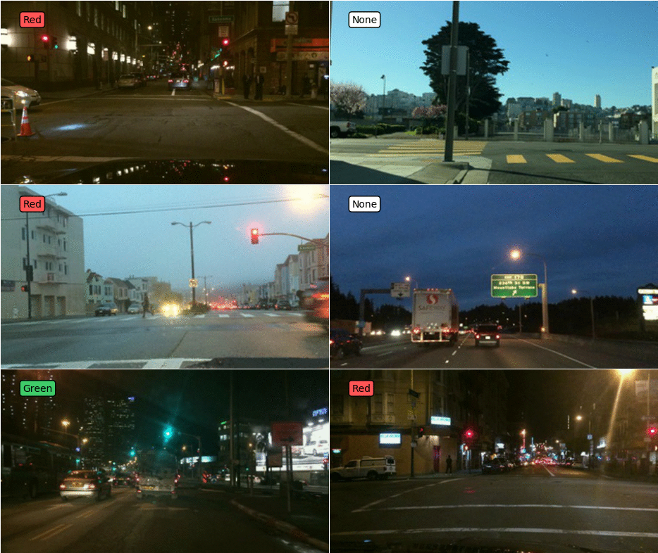
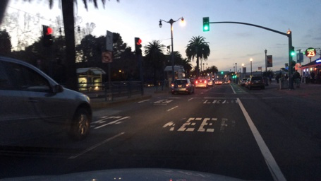
The goal of the challenge was to recognize the traffic light state in images taken by drivers using the Nexar app. In any given image, the classifier needed to output whether there was a traffic light in the scene, and whether it was red or green. More specifically, it should only identify traffic lights in the driving direction.

Here are a few examples to make it clearer:

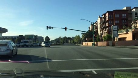
The images above are examples of the three possible classes I needed to predict: no traffic light (left), red traffic light (center) and green traffic light (right).

The challenge required the solution to be based on Convolutional Neural Networks, a very popular method used in image recognition with deep neural networks. The submissions were scored based on the model’s accuracy along with the model’s size (in megabytes). Smaller models got higher scores. In addition, the minimum accuracy required to win was 95%.

Nexar provided 18,659 labeled images as training data. Each image was labeled with one of the three classes mentioned above (no traffic light / red / green).

Software and hardware

I used Caffe to train the models. The main reason I chose Caffe was because of the large variety of pre-trained models.

Python, NumPy & Jupyter Notebook were used for analyzing results, data exploration and ad-hoc scripts.

Amazon’s GPU instances (g2.2xlarge) were used to train the models. My AWS bill ended up being $263 (!). Not cheap. 😑

The code and files I used to train and run the model are on GitHub.

The final classifier

The final classifier achieved an accuracy of 94.955% on Nexar’s test set, with a model size of ~7.84 MB. To compare, GoogLeNet uses a model size of 41 MB, and VGG-16 uses a model size of 528 MB.

Nexar was kind enough to accept 94.955% as 95% to pass the minimum requirement 😁.

The process of getting higher accuracy involved a LOT of trial and error. Some of it had some logic behind it, and some was just “maybe this will work”. I’ll describe some of the things I tried to improve the model that did and didn’t help. The final classifier details are described right after.

What worked?

Transfer learning

I started off with trying to fine-tune a model which was pre-trained on ImageNet with the GoogLeNet architecture. Pretty quickly this got me to >90% accuracy! 😯

Nexar mentioned in the challenge page that it should be possible to reach 93% by fine-tuning GoogLeNet. Not exactly sure what I did wrong there, I might look into it.

SqueezeNet

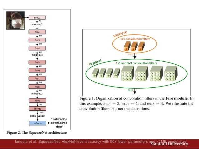
SqueezeNet: AlexNet-level accuracy with 50x fewer parameters and <0.5MB model size.

Since the competition rewards solutions that use small models, early on I decided to look for a compact network with as few parameters as possible that can still produce good results. Most of the recently published networks are very deep and have a lot of parameters. SqueezeNet seemed to be a very good fit, and it also had a pre-trained model trained on ImageNet available in Caffe’s Model Zoo which came in handy.

SqueezeNet network architecture. Slides

The network manages to stay compact by:

  • Using mostly 1x1 convolution filters and some 3x3
  • Reducing number of input channels into the 3x3 filters

For more details, I recommend reading this blog post by Lab41 or the original paper.

After some back and forth with adjusting the learning rate I was able to fine-tune the pre-trained model as well as training from scratch with good accuracy results: 92%! Very cool! 🙌

Rotating images

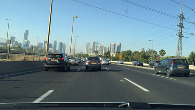
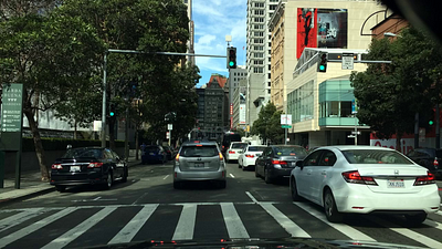
Source: Nexar

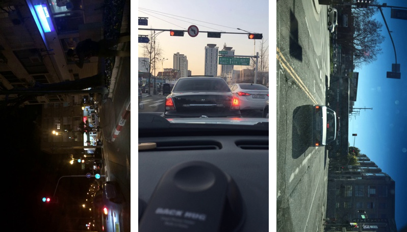
Most of the images were horizontal like the one above, but about 2.4% were vertical, and with all kinds of directions for “up”. See below.

Different orientations of vertical images. Source: Nexar challenge

Although it’s not a big part of the data-set, we want our model classify them correctly too.

Unfortunately, there was no EXIF data in the jpeg images specifying the orientation. At first I considered doing some heuristic to identify the sky and flip the image accordingly, but that did not seem straightforward.

Instead, I tried to make the model invariant to rotations. My first attempt was to train the network with random rotations of 0°, 90°, 180°, 270°. That didn’t help 🤔. But when averaging the predictions of 4 rotations for each image, there was improvement!

92% → 92.6% 👍

To clarify: by “averaging the predictions” I mean averaging the probabilities the model produced of each class across the 4 image variations.

Oversampling crops

During training the SqueezeNet network first performed random cropping on the input images by default, and I didn’t change it. This type of data augmentation makes the network generalize better.

Similarly, when generating predictions, I took several crops of the input image and averaged the results. I used 5 crops: 4 corners and a center crop. The implementation was free by using existing caffe code for this.

92% → 92.46% 👌

Rotating images together with oversampling crops showed very slight improvement.

Additional training with lower learning rate

All models were starting to overfit after a certain point. I noticed this by watching the validation-set loss start to rise at some point.

Validation loss rising from around iteration 40,000

I stopped the training at that point because the model was probably not generalizing any more. This meant that the learning rate didn’t have time to decay all the way to zero. I tried resuming the training process at the point where the model started overfitting with a learning rate 10 times lower than the original one. This usually improved the accuracy by 0-0.5%.

More training data

At first, I split my data into 3 sets: training (64%), validation (16%) & test (20%). After a few days, I thought that giving up 36% of the data might be too much. I merged the training & validations sets and used the test-set to check my results.

I retrained a model with “image rotations” and “additional training at lower rate” and saw improvement:

92.6% → 93.5% 🤘

Relabeling mistakes in the training data

When analyzing the mistakes the classifier had on the validation set, I noticed that some of the mistakes have very high confidence. In other words, the model is certain it’s one thing (e.g. green light) while the training data says another (e.g. red light).

Notice that in the plot above, the right-most bar is pretty high. That means there’s a high number of mistakes with >95% confidence. When examining these cases up close I saw these were usually mistakes in the ground-truth of the training set rather than in the trained model.

I decided to fix these errors in the training set. The reasoning was that these mistakes confuse the model, making it harder for it to generalize. Even if the final testing-set has mistakes in the ground-truth, a more generalized model has a better chance of high accuracy across all the images.

I manually labeled 709 images that one of my models got wrong. This changed the ground-truth for 337 out of the 709 images. It took about an hour of manual work with a python script to help me be efficient.

Above is the same plot after re-labeling and retraining the model. Looks better!

This improved the previous model by:

93.5% → 94.1% ✌️

Ensemble of models

Using several models together and averaging their results improved the accuracy as well. I experimented with different kinds of modifications in the training process of the models involved in the ensemble. A noticeable improvement was achieved by using a model trained from scratch even though it had lower accuracy on its own together with the models that were fine-tuned on pre-trained models. Perhaps this is because this model learned different features than the ones that were fine-tuned on pre-trained models.

The ensemble used 3 models with accuracies of 94.1%, 94.2% and 92.9% and together got an accuracy of 94.8%. 👾

What didn’t work?

Lots of things! 🤕 Hopefully some of these ideas can be useful in other settings.

Combatting overfitting

While trying to deal with overfitting I tried several things, none of which produced significant improvements:

  • increasing the dropout ratio in the network
  • more data augmentation (random shifts, zooms, skews)
  • training on more data: using 90/10 split instead of 80/20

Balancing the dataset

The dataset wasn’t very balanced:

  • 19% of images were labeled with no traffic light
  • 53% red light
  • 28% green light.

I tried balancing the dataset by oversampling the less common classes but didn’t notice any improvement.

Separating day & night

My intuition was that recognizing traffic lights in daylight and nighttime is very different. I thought maybe I could help the model by separating it into two simpler problems.

It was fairly easy to separate the images to day and night by looking at their average pixel intensity:

You can see a very natural separation of images with low average values, i.e. dark images, taken at nighttime, and bright images, taken at daytime.

I tried two approaches, both didn’t improve the results:

  • Training two separate models for day images and night images
  • Training the network to predict 6 classes instead of 3 by also predicting whether it’s day or night

Using better variants of SqueezeNet

I experimented a little bit with two improved variants of SqueezeNet. The first used residual connections and the second was trained with dense→sparse→dense training (more details in the paper). No luck. 😕

Localization of traffic lights

After reading a great post by deepsense.io on how they won the whale recognition challenge, I tried to train a localizer, i.e. identify the location of the traffic light in the image first, and then identify the traffic light state on a small region of the image.

I used sloth to annotate about 2,000 images which took a few hours. When trying to train a model, it was overfitting very quickly, probably because there was not enough labeled data. Perhaps this could work if I had annotated a lot more images.

Training a classifier on the hard cases

I chose 30% of the “harder” images by selecting images which my classifier was less than 97% confident about. I then tried to train classifier just on these images. No improvement. 😑

Different optimization algorithm

I experimented very shortly with using Caffe’s Adam solver instead of SGD with linearly decreasing learning rate but didn’t see any improvement. 🤔

Adding more models to ensemble

Since the ensemble method proved helpful, I tried to double-down on it. I tried changing different parameters to produce different models and add them to the ensemble: initial seed, dropout rate, different training data (different split), different checkpoint in the training. None of these made any significant improvement. 😞

Final classifier details

The classifier uses an ensemble of 3 separately trained networks. A weighted average of the probabilities they give to each class is used as the output. All three networks were using the SqueezeNet network but each one was trained differently.

Model #1 — Pre-trained network with oversampling

Trained on the re-labeled training set (after fixing the ground-truth mistakes). The model was fine-tuned based on a pre-trained model of SqueezeNet trained on ImageNet.

Data augmentation during training:

  • Random horizontal mirroring
  • Randomly cropping patches of size 227 x 227 before feeding into the network

At test time, the predictions of 10 variations of each image were averaged to calculate the final prediction. The 10 variations were made of:

  • 5 crops of size 227 x 227: 1 for each corner and 1 in the center of the image
  • for each crop, a horizontally mirrored version was also used

Model accuracy on validation set: 94.21%
Model size: ~2.6 MB

Model #2 — Adding rotation invariance

Very similar to Model #1, with the addition of image rotations. During training time, images were randomly rotated by 90°, 180°, 270° or not at all. At test-time, each one of the 10 variations described in Model #1 created three more variations by rotating it by 90°, 180° and 270°. A total of 40 variations were classified by our model and averaged together.

Model accuracy on validation set: 94.1%
Model size: ~2.6 MB

Model #3 — Trained from scratch

This model was not fine-tuned, but instead trained from scratch. The rationale behind it was that even though it achieves lower accuracy, it learns different features on the training set than the previous two models, which could be useful when used in an ensemble.

Data augmentation during training and testing are the same as Model #1: mirroring and cropping.

Model accuracy on validation set: 92.92%
Model size: ~2.6 MB

Combining the models together

Each model output three values, representing the probability that the image belongs to each one of the three classes. We averaged their outputs with the following weights:

  • Model #1: 0.28
  • Model #2: 0.49
  • Model #3: 0.23

The values for the weights were found by doing a grid-search over possible values and testing it on the validation set. They are probably a little overfitted to the validation set, but perhaps not too much since this is a very simple operation.

Model accuracy on validation set: 94.83%
Model size: ~7.84 MB
Model accuracy on Nexar’s test set: 94.955% 🎉

Examples of the model mistakes

Source: Nexar

The green dot in the palm tree produced by the glare probably made the model predict there’s a green light by mistake.

Source: Nexar

The model predicted red instead of green. Tricky case when there is more than one traffic light in the scene.

The model said there’s no traffic light while there’s a green traffic light ahead.

Conclusion

This was the first time I applied deep learning on a real problem! I was happy to see it worked so well. I learned a LOT during the process and will probably write another post that will hopefully help newcomers waste less time on some of the mistakes and technical challenges I had.

I want to thank Nexar for providing this great challenge and hope they organize more of these in the future! 🙌


If you enjoyed reading this post, please tap below!

Would love to get your feedback and questions below!


Posted by uniqueone
,