Keras Tutorial: The Ultimate Beginner's Guide to Deep Learning in Python
https://elitedatascience.com/keras-tutorial-deep-learning-in-python
Posted by uniqueone
,

Practical Deep Learning For Coders—18 hours of lessons for free
http://course.fast.ai/
Posted by uniqueone
,
텐서플로우도 좋지만, 컴퓨터사이언스가 전공이 아니고
기존 알고리즘들의 응용을 목적으로 하는 (저와 같은) 사람들을 위해서는 Keras로도 충분하다고 생각합니다 (제 전공은 산업공학입니다..)

그래서 Keras를 공부중인데 자료가 많이 없더라구요.

구글링해서 찾은 Keras CNN 튜토리얼을
https://elitedatascience.com/keras-tutorial-deep-learning-in-python
제 환경에 맞게(최신 Keras의 변경점을 수정하여)

나름대로 정리해봤습니다
https://byeongkijeong.github.io/Keras-cnn-tutorial/

Keras의 Backend를 Tensorflow로 사용하니, 본 그룹에 위배되지 않을거라 생각합니다 ㅎㅎ

블로그도, Jekyll도 처음이고 Markdown도 처음이라
글이 지저분하네요.

조만간 수정해보겠습니다 ㅠㅠ
Posted by uniqueone
,
입력 값에서 답을 찾아내는 sequence-to-sequence 모델인 "Pointer Networks" https://arxiv.org/abs/1506.03134 를 TensorFlow로 구현했습니다.

https://github.com/devsisters/pointer-network-tensorflow

논문은 랜덤한 점들을 모두 한번씩만 방문하고 출발 도시로 돌아오는 최단 거리를 찾는 Travelling Salesman Problem(TSP)처럼 입력 값에서 정해진 순서로 답을 찾아야 하는 문제를 풀 수 있는 모델을 제안했습니다.

2015년 6월에 arxiv에 올라온 논문이지만 굉장히 유용한 모델 중 하나라 생각되어 구현하게 되었습니다. 이번에는 I/O 시간을 최소화 하기 위해서 멀티스레드로 데이터 큐를 따로 두어 TensorFlow graph의 실행이 I/O에 방해받지 않도록 구현했습니다.

===

그리고 제가 현재 학사 병특 중인 데브시스터즈에서 함께 일할 머신러닝 리서쳐를 찾고 있습니다 :)

저희 회사에서는 강화학습, Computer vision, NLP 등 자신이 풀고자 하는 문제를 자유롭게 정하고 논문 세미나와 코드 구현을 통해서 팀의 역량을 키워나가고 있습니다. 관심이 있으신 분들은 언제든지 연락주세요!

지원 방법 : http://www.devsisters.com/jobs
채용 문의 : career@devsisters.com

저희 팀의 외부 발표자료 및 오픈소스 프로젝트를 공유합니다.

- 딥러닝과 강화 학습으로 나보다 잘하는 쿠키런 AI 구현하기 http://www.slideshare.net/carpedm20/ai-67616630
- 텐서플로우 설치도 했고 튜토리얼도 봤고 기초 예제도 짜봤다면 http://www.slideshare.net/carpedm20/ss-63116251
- 지적 대화를 위한 깊고 넓은 딥러닝 http://www.slideshare.net/carpedm20/pycon-korea-2016
- 강화 학습 기초 http://www.slideshare.net/carpedm20/reinforcement-learning-an-introduction-64037079

- 애플의 Simulated+Unsupervised (S+U) learning 구현 https://github.com/carpedm20/simulated-unsupervised-tensorflow
- Neural Combinatorial Optimization 구현 https://github.com/devsisters/neural-combinatorial-rl-tensorflow
- Deep Q-network 구현 https://github.com/devsisters/DQN-tensorflow
Posted by uniqueone
,
grad-cam.tensorflow

Implementation of Grad CAM in tensorflow

Gradient class activation maps are a visualization technique for deep learning networks.
https://github.com/Ankush96/grad-cam.tensorflow

also:

Grad-CAM implementation in Keras
https://github.com/jacobgil/keras-grad-cam

Grad-CAM: Gradient-weighted Class Activation Mapping
https://github.com/ramprs/grad-cam (torch)
Posted by uniqueone
,
http://bcho.tistory.com/m/1156
Posted by uniqueone
,

https://youtu.be/r7-WPbx8VuY
Posted by uniqueone
,

https://youtu.be/BtDgICVvkHE
Posted by uniqueone
,


https://github.com/BinRoot/TensorFlow-Book?utm_content=buffer3f3de&utm_medium=social&utm_source=twitter.com&utm_campaign=buffer


Machine Learning with TensorFlow

This is the official code repository for Machine Learning with TensorFlow.

:warning: Warning: The book will be released in a month or two, so this repo is a pre-release of the entire code. I will be heavily updating this repo in the coming weeks. Stay tuned, and follow along! :)

Get started with machine learning using TensorFlow, Google's latest and greatest machine learning library.

Summary

Chapter 2 - TensorFlow Basics

  • Concept 1: Defining tensors
  • Concept 2: Evaluating ops
  • Concept 3: Interactive session
  • Concept 4: Session loggings
  • Concept 5: Variables
  • Concept 6: Saving variables
  • Concept 7: Loading variables
  • Concept 8: TensorBoard

Chapter 3 - Regression

  • Concept 1: Linear regression
  • Concept 2: Polynomial regression
  • Concept 3: Regularization

Chapter 4 - Classification

  • Concept 1: Linear regression for classification
  • Concept 2: Logistic regression
  • Concept 3: 2D Logistic regression
  • Concept 4: Softmax classification

Chapter 5 - Clustering

  • Concept 1: Clustering
  • Concept 2: Segmentation
  • Concept 3: Self-organizing map

Chapter 6 - Hidden markov models

  • Concept 1: Forward algorithm
  • Concept 2: Viterbi decode

Chapter 7 - Autoencoders

  • Concept 1: Autoencoder
  • Concept 2: Applying an autoencoder to images
  • Concept 3: Denoising autoencoder

Chapter 8 - Reinforcement learning

  • Concept 1: Reinforcement learning

Chapter 9 - Convolutional Neural Networks

  • Concept 1: Using CIFAR-10 dataset
  • Concept 2: Convolutions
  • Concept 3: Convolutional neural network

Chapter 10 - Recurrent Neural Network

  • Concept 1: Loading timeseries data
  • Concept 2: Recurrent neural networks
  • Concept 3: Applying RNN to real-world data for timeseries prediction
Posted by uniqueone
,

http://warmspringwinds.github.io/tensorflow/tf-slim/2016/10/30/image-classification-and-segmentation-using-tensorflow-and-tf-slim/


A post showing how to perform Image Classification and Image Segmentation with a recently released TF-Slim library and pretrained models.


Inroduction

In this post I want to show an example of application of Tensorflow and a recently released library slim for Image Classification, Image Annotation and Segmentation. In the post I focus on slim, cover a small theoretical part and show possible applications.

I have tried other libraries before like Caffe, Matconvnet, Theano and Torch. All of them have their pros and cons, but I always wanted a library in Python that is flexible, has good support and has a lot of pretrained models. Recently, a new library called slim was released along with a set of standart pretrained models like ResNet, VGG, Inception-ResNet-v2 (new winner of ILSVRC) and others. This library along with models are supported by Google, which makes it even better. There was a need for a library like this because Tensorflow itself is a very low-level and any implementation can become highly complicated. It requires writing a lot of boilerplate code. Reading other people’s code was also complicated. slim is a very clean and lightweight wrapper around Tensorflow with pretrained models.

This post assumes a prior knowledge of Tensorflow and Convolutional Neural Networks. Tensorflow has a nice tutorials on both of these. You can find them here.

The blog post is created using jupyter notebook. After each chunk of a code you can see the result of its evaluation. You can also get the notebook file from here. The content of the blog post is partially borrowed from slim walkthough notebook.

Setup

To be able to run the code, you will need to have Tensorflow installed. I have used r0.11. You will need to have tensorflow/models repository cloned. To clone it, simply run:

git clone https://github.com/tensorflow/models

I am also using scikit-image library and numpy for this tutorial plus other dependencies. One of the ways to install them is to download Anaconda software package for python.

First, we specify tensorflow to use the first GPU only. Be careful, by default it will use all available memory. Second, we need to add the cloned repository to the path, so that python is able to see it.

import sys
import os

os.environ["CUDA_VISIBLE_DEVICES"] = '0'
sys.path.append("/home/dpakhom1/workspace/models/slim")

Now, let’s download the VGG-16 model which we will use for classification of images and segmentation. You can also use networks that will consume less memory(for example, AlexNet). For more models look here.

from datasets import dataset_utils
import tensorflow as tf

url = "http://download.tensorflow.org/models/vgg_16_2016_08_28.tar.gz"

# Specify where you want to download the model to
checkpoints_dir = '/home/dpakhom1/checkpoints'

if not tf.gfile.Exists(checkpoints_dir):
    tf.gfile.MakeDirs(checkpoints_dir)

dataset_utils.download_and_uncompress_tarball(url, checkpoints_dir)
>> Downloading vgg_16_2016_08_28.tar.gz 100.0%
Successfully downloaded vgg_16_2016_08_28.tar.gz 513324920 bytes.

Image Classification

The model that we have just downloaded was trained to be able to classify images into 1000 classes. The set of classes is very diverse. In our blog post we will use the pretrained model to classify, annotate and segment images into these 1000 classes.

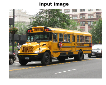
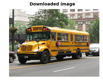
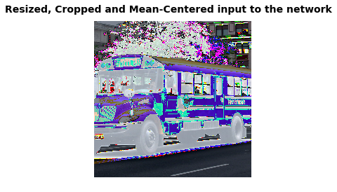
Below you can see an example of Image Classification. We preprocess the input image by resizing it while preserving the aspect ratio and crop the central part. The size of the crop is equal to the size of images that the network was trained on.

%matplotlib inline

from matplotlib import pyplot as plt

import numpy as np
import os
import tensorflow as tf
import urllib2

from datasets import imagenet
from nets import vgg
from preprocessing import vgg_preprocessing

checkpoints_dir = '/home/dpakhom1/checkpoints'

slim = tf.contrib.slim

# We need default size of image for a particular network.
# The network was trained on images of that size -- so we
# resize input image later in the code.
image_size = vgg.vgg_16.default_image_size


with tf.Graph().as_default():
    
    url = ("https://upload.wikimedia.org/wikipedia/commons/d/d9/"
           "First_Student_IC_school_bus_202076.jpg")
    
    # Open specified url and load image as a string
    image_string = urllib2.urlopen(url).read()
    
    # Decode string into matrix with intensity values
    image = tf.image.decode_jpeg(image_string, channels=3)
    
    # Resize the input image, preserving the aspect ratio
    # and make a central crop of the resulted image.
    # The crop will be of the size of the default image size of
    # the network.
    processed_image = vgg_preprocessing.preprocess_image(image,
                                                         image_size,
                                                         image_size,
                                                         is_training=False)
    
    # Networks accept images in batches.
    # The first dimension usually represents the batch size.
    # In our case the batch size is one.
    processed_images  = tf.expand_dims(processed_image, 0)
    
    # Create the model, use the default arg scope to configure
    # the batch norm parameters. arg_scope is a very conveniet
    # feature of slim library -- you can define default
    # parameters for layers -- like stride, padding etc.
    with slim.arg_scope(vgg.vgg_arg_scope()):
        logits, _ = vgg.vgg_16(processed_images,
                               num_classes=1000,
                               is_training=False)
    
    # In order to get probabilities we apply softmax on the output.
    probabilities = tf.nn.softmax(logits)
    
    # Create a function that reads the network weights
    # from the checkpoint file that you downloaded.
    # We will run it in session later.
    init_fn = slim.assign_from_checkpoint_fn(
        os.path.join(checkpoints_dir, 'vgg_16.ckpt'),
        slim.get_model_variables('vgg_16'))
    
    with tf.Session() as sess:
        
        # Load weights
        init_fn(sess)
        
        # We want to get predictions, image as numpy matrix
        # and resized and cropped piece that is actually
        # being fed to the network.
        np_image, network_input, probabilities = sess.run([image,
                                                           processed_image,
                                                           probabilities])
        probabilities = probabilities[0, 0:]
        sorted_inds = [i[0] for i in sorted(enumerate(-probabilities),
                                            key=lambda x:x[1])]
    
    # Show the downloaded image
    plt.figure()
    plt.imshow(np_image.astype(np.uint8))
    plt.suptitle("Downloaded image", fontsize=14, fontweight='bold')
    plt.axis('off')
    plt.show()
    
    # Show the image that is actually being fed to the network
    # The image was resized while preserving aspect ratio and then
    # cropped. After that, the mean pixel value was subtracted from
    # each pixel of that crop. We normalize the image to be between [-1, 1]
    # to show the image.
    plt.imshow( network_input / (network_input.max() - network_input.min()) )
    plt.suptitle("Resized, Cropped and Mean-Centered input to network",
                 fontsize=14, fontweight='bold')
    plt.axis('off')
    plt.show()

    names = imagenet.create_readable_names_for_imagenet_labels()
    for i in range(5):
        index = sorted_inds[i]
        # Now we print the top-5 predictions that the network gives us with
        # corresponding probabilities. Pay attention that the index with
        # class names is shifted by 1 -- this is because some networks
        # were trained on 1000 classes and others on 1001. VGG-16 was trained
        # on 1000 classes.
        print('Probability %0.2f => [%s]' % (probabilities[index], names[index+1]))
        
    res = slim.get_model_variables()

png

png

Probability 1.00 => [school bus]
Probability 0.00 => [minibus]
Probability 0.00 => [passenger car, coach, carriage]
Probability 0.00 => [trolleybus, trolley coach, trackless trolley]
Probability 0.00 => [cab, hack, taxi, taxicab]

Image Annotation and Segmentation

As you can see from the previous example, only a certain part of the original image is being processed by the network. This is good only for cases when we want to get a single prediction for an image.

Sometimes we want to get more information from an image. For example, it would be great to know about all the objects that are present in the image. For example, network would tell us that it found a school bus, other cars and building. Using this information, we can create a search engine that will be able to give us all images that has a particular object in them. This can be seen as a simple case of Image Annotation.

But what if we also want to get spatial information about the objects locations. Can the network tell us that it sees a bus in the center of the image and building on the top-right corner? That way we can create a more specific queries for a search engine: “Give me all images where the school bus is located in the middle AND flower pot in the top left corner”.

There are cases when we need to classify each pixel of the image, also know as the task of Segmentation. Imagine, that we have a huge dataset with pictures and we want to blur faces of people there, so that we don’t have to get their permission to publish these pictures. For example, you can see people’s faces being blured in Google Street View. But we only need to blur faces and not other content that might be important. Segmentation can help us in this case. We can get pixels that belong to faces and blur only them.

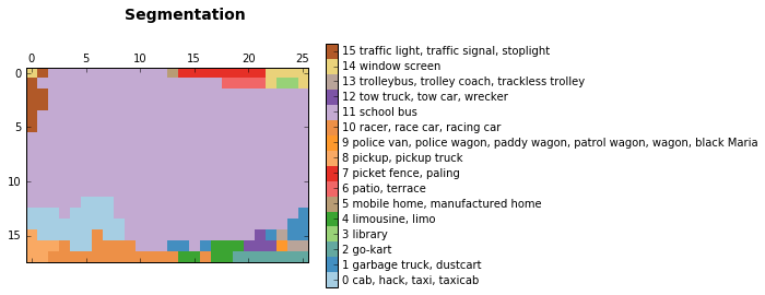
Below we will see a simple example of Segmentation. For the simplicity, the segmentation will be of a smaller size than the original image. We can do segmentation using an existing Convolutional Neural Network by applying it in a Fully Convolutional manner. This is done by casting the Fully Connected Layers of a network into Convolutional – this way we can input image of any size and get segmentation of lower resolution due to max-pooling layers that are used in network. To get the Segmentation of the same size as an input, deconvolutional layers can be used. You can read more about this in the paper fully convolutional networks for semantic segmentation by Long et al. We won’t consider deconvolutional layers in this example. Example below shows how to get segmentation of lower resolution than the input. Deconvolutional layers can be seen as a way to perform interpolation. Interpolation can be different (quadratic, qubic and other) but network can learn a specific interpolation that performs well under a certain task.

from preprocessing import vgg_preprocessing

# Load the mean pixel values and the function
# that performs the subtraction
from preprocessing.vgg_preprocessing import (_mean_image_subtraction,
                                            _R_MEAN, _G_MEAN, _B_MEAN)

# Function to nicely print segmentation results with
# colorbar showing class names
def discrete_matshow(data, labels_names=[], title=""):
    #get discrete colormap
    cmap = plt.get_cmap('Paired', np.max(data)-np.min(data)+1)
    # set limits .5 outside true range
    mat = plt.matshow(data,
                      cmap=cmap,
                      vmin = np.min(data)-.5,
                      vmax = np.max(data)+.5)
    #tell the colorbar to tick at integers
    cax = plt.colorbar(mat,
                       ticks=np.arange(np.min(data),np.max(data)+1))
    
    # The names to be printed aside the colorbar
    if labels_names:
        cax.ax.set_yticklabels(labels_names)
    
    if title:
        plt.suptitle(title, fontsize=14, fontweight='bold')


with tf.Graph().as_default():
    
    url = ("https://upload.wikimedia.org/wikipedia/commons/d/d9/"
           "First_Student_IC_school_bus_202076.jpg")
    
    image_string = urllib2.urlopen(url).read()
    image = tf.image.decode_jpeg(image_string, channels=3)
    
    # Convert image to float32 before subtracting the
    # mean pixel value
    image_float = tf.to_float(image, name='ToFloat')
    
    # Subtract the mean pixel value from each pixel
    processed_image = _mean_image_subtraction(image_float,
                                              [_R_MEAN, _G_MEAN, _B_MEAN])

    input_image = tf.expand_dims(processed_image, 0)
    
    with slim.arg_scope(vgg.vgg_arg_scope()):
        
        # spatial_squeeze option enables to use network in a fully
        # convolutional manner
        logits, _ = vgg.vgg_16(input_image,
                               num_classes=1000,
                               is_training=False,
                               spatial_squeeze=False)
    
    # For each pixel we get predictions for each class
    # out of 1000. We need to pick the one with the highest
    # probability. To be more precise, these are not probabilities,
    # because we didn't apply softmax. But if we pick a class
    # with the highest value it will be equivalent to picking
    # the highest value after applying softmax
    pred = tf.argmax(logits, dimension=3)
    
    init_fn = slim.assign_from_checkpoint_fn(
        os.path.join(checkpoints_dir, 'vgg_16.ckpt'),
        slim.get_model_variables('vgg_16'))
    
    with tf.Session() as sess:
        init_fn(sess)
        segmentation, np_image = sess.run([pred, image])

# Remove the first empty dimension
segmentation = np.squeeze(segmentation)

# Let's get unique predicted classes (from 0 to 1000) and
# relable the original predictions so that classes are
# numerated starting from zero
unique_classes, relabeled_image = np.unique(segmentation,
                                            return_inverse=True)

segmentation_size = segmentation.shape

relabeled_image = relabeled_image.reshape(segmentation_size)

labels_names = []

for index, current_class_number in enumerate(unique_classes):

    labels_names.append(str(index) + ' ' + names[current_class_number+1])

discrete_matshow(data=relabeled_image, labels_names=labels_names, title="Segmentation")

png

png

The segmentation that was obtained shows that network was able to find the school bus, traffic sign in the left-top corner that can’t be clearly seen in the image. It was able to locate windows at the top-left corner and even made a hypothesis that it is a library (we don’t know if that is true). It also made a certain number of not so correct predictions. Those are usually caused by the fact that the network can only see a part of image when it is centered at a pixel. The characteristic of a network that represents it is called receptive field. Receptive field of the network that we use in this blog is 404 pixels. So when network can only see a part of the school bus, it confuses it with taxi or pickup truck. You can see that in the bottom-left corner of segmentation results.

As we can see above, we got a simple segmentation for our image. It is not very precise because the network was originally trained to perform classification and not segmentation. If we want to get better results, we will have to train it ourselves. Anyways, the results that we got are suitable for image annotation and very approximate segmentation.

Performing Segmentation using Convolutional Neural Networks can be seen as performing classification at different parts of an input image. We center network at a particular pixel, make prediction and assign label to that pixel. This way we add spatial information to our classification and get segmentation.

Conclusion and Discussion

In this blog post we covered slim library by performing Image Classification and Segmentation. The post also explains a certain amount of theory behind both tasks.

In my opinion, slim along with pretrained models can be a very powerful tool while remaining very flexible and you can always intermix Tensorflow with it. It is relatively new, therefore, it lacks documentation and sometimes you have to read the source code. It has support from Google and is currently in an active development.

Posted by uniqueone
,

https://elitedatascience.com/keras-tutorial-deep-learning-in-python


In this step-by-step Keras tutorial, you’ll learn how to build a convolutional neural network in Python!

In fact, we’ll be training a classifier for handwritten digits that boasts over 99% accuracy on the famous MNIST dataset.

Before we begin, we should note that this guide is geared toward beginners who are interested in applied deep learning.

Our goal is to introduce you to one of the most popular and powerful libraries for building neural networks in Python. That means we’ll brush over much of the theory and math, but we’ll also point you to great resources for learning those.

Keras Tutorial

Before we start...

Recommended Prerequisites

The recommended prerequisites for this guide are:

To move quickly, we'll assume you have this background.

Why Keras?

Keras is our recommended library for deep learning in Python, especially for beginners. Its minimalistic, modular approach makes it a breeze to get deep neural networks up and running. You can read more about it here:

WTF is Deep Learning?

Deep learning refers to neural networks with multiple hidden layers that can learn increasingly abstract representations of the input data. This is obviously an oversimplification, but it's a practical definition for us right now.

For example, deep learning has led to major advances in computer vision. We're now able to classify images, find objects in them, and even label them with captions. To do so, deep neural networks with many hidden layers can sequentially learn more complex features from the raw input image:

  • The first hidden layers might only learn local edge patterns.
  • Then, each subsequent layer (or filter) learns more complex representations.
  • Finally, the last layer can classify the image as a cat or kangaroo.

These types of deep neural networks are called Convolutional Neural Networks.

WTF are Convolutional Neural Networks?

In a nutshell, Convolutional Neural Networks (CNN's) are multi-layer neural networks (sometimes up to 17 or more layers) that assume the input data to be images.

Typical CNN Architecture

Typical CNN Architecture

By making this requirement, CNN's can drastically reduce the number of parameters that need to be tuned. Therefore, CNN's can efficiently handle the high dimensionality of raw images.

Their underlying mechanics are beyond the scope of this tutorial, but you can read more about them here.

What this tutorial is not:

This is not a complete course on deep learning. Instead, this tutorial is meant to get you from zero to your first Convolutional Neural Network with as little headache as possible!

If you're interested in mastering the theory behind deep learning, we recommend this great course from Stanford:

A quick tip before we begin:

We tried to make this tutorial as streamlined as possible, which means we won't go into too much detail for any one topic. It's helpful to have the Keras documentation open beside you, in case you want to learn more about a function or module.

Keras Tutorial Contents

Here are the steps for building your first CNN using Keras:

  1. Set up your environment.
  2. Install Keras.
  3. Import libraries and modules.
  4. Load image data from MNIST.
  5. Preprocess input data for Keras.
  6. Preprocess class labels for Keras.
  7. Define model architecture.
  8. Compile model.
  9. Fit model on training data.
  10. Evaluate model on test data.

Step 1: Set up your environment.

First, hang up a motivational poster:

Motivational poster

Probably useless.

Next, make sure you have the following installed on your computer:

  • Python 2.7+ (Python 3 is fine too, but Python 2.7 is still more popular for data science overall)
  • SciPy with NumPy
  • Matplotlib (Optional, recommended for exploratory analysis)
  • Theano* (Installation instructions)

We strongly recommend installing Python, NumPy, SciPy, and matplotlib through the Anaconda Distribution. It comes with all of those packages.

*note: TensorFlow is also supported (as an alternative to Theano), but we stick with Theano to keep it simple. The main difference is that you'll need to reshape the data slightly differently before feeding it to your network.

You can check to see if you've installed everything correctly:

Go to your command line program (Terminal on a Mac) and type in:

You'll see the Python interpreter:

Next, you can import your libraries and print their versions:


Step 2: Install Keras.

It wouldn't be a Keras tutorial if we didn't cover how to install Keras.

The good news is that if you used Anaconda, then you'll already have a nice package management system called pip installed.

You can confirm you have it installed by typing  $ pip in your command line. It should output a list of commands and options. If you don't have pip, you can install it here.

Once you have pip, installing Keras is easy as pie:

You can confirm it's installed correctly:

Oops... looks like that Keras version is outdated. Upgrading the version is easy:

Perfect, now let's start a new Python file and name it keras_cnn_example.py.

Step 3: Import libraries and modules.

Let's start by importing numpy and setting a seed for the computer's pseudorandom number generator. This allows us to reproduce the results from our script:

Next, we'll import the Sequential model type from Keras. This is simply a linear stack of neural network layers, and it's perfect for the type of feed-forward CNN we're building in this tutorial.

Next, let's import the "core" layers from Keras. These are the layers that are used in almost any neural network:

Then, we'll import the CNN layers from Keras. These are the convolutional layers that will help us efficiently train on image data:

Finally, we'll import some utilities. This will help us transform our data later:

Now we have everything we need to build our neural network architecture.

Step 4: Load image data from MNIST.

MNIST is a great dataset for getting started with deep learning and computer vision. It's a big enough challenge to warrant neural networks, but it's manageable on a single computer. We discuss it more in our post: 6 Fun Machine Learning Projects for Beginners.

The Keras library conveniently includes it already. We can load it like so:

We can look at the shape of the dataset:

Great, so it appears that we have 60,000 samples in our training set, and the images are 28 pixels x 28 pixels each. We can confirm this by plotting the first sample in matplotlib:

And here's the image output:

MNIST Digit

In general, when working with computer vision, it's helpful to visually plot the data before doing any algorithm work. It's a quick sanity check that can prevent easily avoidable mistakes (such as misinterpreting the data dimensions).

Step 5: Preprocess input data for Keras.

When using the Theano backend, you must explicitly declare a dimension for the depth of the input image. For example, a full-color image with all 3 RGB channels will have a depth of 3.

Our MNIST images only have a depth of 1, but we must explicitly declare that.

In other words, we want to transform our dataset from having shape (n, width, height) to (n, depth, width, height).

Here's how we can do that easily:

To confirm, we can print X_train's dimensions again:

The final preprocessing step for the input data is to convert our data type to float32 and normalize our data values to the range [0, 1].

Now, our input data are ready for model training.

Step 6: Preprocess class labels for Keras.

Next, let's take a look at the shape of our class label data:

Hmm... that may be problematic. We should have 10 different classes, one for each digit, but it looks like we only have a 1-dimensional array. Let's take a look at the labels for the first 10 training samples:

And there's the problem. The y_train and y_test data are not split into 10 distinct class labels, but rather are represented as a single array with the class values.

We can fix this easily:

Now we can take another look:

There we go... much better!

Step 7:  Define model architecture.

Now we're ready to define our model architecture. In actual R&D work, researchers will spend a considerable amount of time studying model architectures.

To keep this tutorial moving along, we're not going to discuss the theory or math here. This alone is a rich and meaty field, and we recommend the CS231n class mentioned earlier for those who want to learn more.

Plus, when you're just starting out, you can just replicate proven architectures from academic papers or use existing examples. Here's a list of example implementations in Keras.

Let's start by declaring a sequential model format:

Next, we declare the input layer:

The input shape parameter should be the shape of 1 sample. In this case, it's the same (1, 28, 28) that corresponds to  the (depth, width, height) of each digit image.

But what do the first 3 parameters represent? They correspond to the number of convolution filters to use, the number of rows in each convolution kernel, and the number of columns in each convolution kernel, respectively.

*Note: The step size is (1,1) by default, and it can be tuned using the 'subsample' parameter.

We can confirm this by printing the shape of the current model output:

Next, we can simply add more layers to our model like we're building legos:

Again, we won't go into the theory too much, but it's important to highlight the Dropout layer we just added. This is a method for regularizing our model in order to prevent overfitting. You can read more about it here.

MaxPooling2D is a way to reduce the number of parameters in our model by sliding a 2x2 pooling filter across the previous layer and taking the max of the 4 values in the 2x2 filter.

So far, for model parameters, we've added two Convolution layers. To complete our model architecture, let's add a fully connected layer and then the output layer:

For Dense layers, the first parameter is the output size of the layer. Keras automatically handles the connections between layers.

Note that the final layer has an output size of 10, corresponding to the 10 classes of digits.

Also note that the weights from the Convolution layers must be flattened (made 1-dimensional) before passing them to the fully connected Dense layer.

Here's how the entire model architecture looks together:

Now all we need to do is define the loss function and the optimizer, and then we'll be ready to train it.

Step 8: Compile model.

Now we're in the home stretch! The hard part is already over.

We just need to compile the model and we'll be ready to train it. When we compile the model, we declare the loss function and the optimizer (SGD, Adam, etc.).

Keras has a variety of loss functions and out-of-the-box optimizers to choose from.

Step 9: Fit model on training data.

To fit the model, all we have to do is declare the batch size and number of epochs to train for, then pass in our training data.

Easy, huh?

You can also use a variety of callbacks to set early-stopping rules, save model weights along the way, or log the history of each training epoch.

Step 10: Evaluate model on test data.

Finally, we can evaluate our model on the test data:

Congratulations... you've made it to the end of this Keras tutorial!

We've just completed a whirlwind tour of Keras's core functionality, but we've only really scratched the surface. Hopefully you've gained the foundation to further explore all that Keras has to offer.

For continued learning, we recommend studying other example models in Keras and Stanford's computer vision class.

The complete code, from start to finish.

Here's all the code in one place, in a single script.

Enjoyed the tutorial?

Sign up for our newsletter for more content like this. You’ll also get instant access to a free PDF guide: Supercharge Your Data Science Career: 88 Free, Hand-Picked Resources Every Data Scientist Should Have.
Posted by uniqueone
,

텐서플로우 관련 좋은 강의 자료가 있어 공유합니다.

Tensorflow and deeplearning without at Ph.D

동영상 강의 : https://youtu.be/vq2nnJ4g6N0
강의 슬라이드 : https://docs.google.com/presentation/d/1TVixw6ItiZ8igjp6U17tcgoFrLSaHWQmMOwjlgQY9co/pub?slide=id.p
GitHub : https://github.com/martin-gorner/tensorflow-mnist-tutorial

Posted by uniqueone
,

안녕하세요 ㅎㅎ TensorFlow KR에는 글을 처음 써보네요!

제가 듣는 대학원 수업에서 발표한 TensorFlow Tutorial 슬라이드와 소스코드 공유합니다 ㅎㅎ

내용은 거의 "텐서플로 첫걸음" 책을 요약한 것입니다 ㅎㅎ 소스 코드도 거의 책의 예제 코드에서 가져왔구요.

...

슬라이드의 특징은:
- MNIST CNN 예제 코드를 그림으로 이쁘게 그림!
- TensorFlow의 MNIST CNN 예제 코드와 동일한 NN을 TFLearn를 사용하여 구현해봄!

이렇게 두 가지 정도입니다 ㅎㅎ

누군가에게 도움이 되었으면 좋겠습니다. 감사합니다.

SlideShare:
http://www.slideshare.net/JunK…/tensorflow-tutorial-68885890

Jupyter Notebook source code:
https://github.com/uosdmlab/tensorflow-tutorial

Posted by uniqueone
,
https://tensorflowkorea.gitbooks.io/tensorflow-kr/content/g3doc/get_started/


텐서플로우를 실제로 작동시켜 봅시다!

시작하기 전에 앞으로 무엇을 배울지 힌트를 얻기위해 파이썬 API로 된 텐서플로우 코드를 잠깐 보겠습니다.

이 코드는 2차원 샘플 데이터를 사용하여 분포에 맞는 직선을 찾는(역주: 회귀분석) 간단한 파이썬 프로그램입니다.


import tensorflow as tf
import numpy as np

# Create 100 phony x, y data points in NumPy, y = x * 0.1 + 0.3
x_data = np.random.rand(100).astype(np.float32)
y_data = x_data * 0.1 + 0.3

# Try to find values for W and b that compute y_data = W * x_data + b
# (We know that W should be 0.1 and b 0.3, but Tensorflow will
# figure that out for us.)
W = tf.Variable(tf.random_uniform([1], -1.0, 1.0))
b = tf.Variable(tf.zeros([1]))
y = W * x_data + b

# Minimize the mean squared errors.
loss = tf.reduce_mean(tf.square(y - y_data))
optimizer = tf.train.GradientDescentOptimizer(0.5)
train = optimizer.minimize(loss)

# Before starting, initialize the variables.  We will 'run' this first.
init = tf.initialize_all_variables()

# Launch the graph.
sess = tf.Session()
sess.run(init)

# Fit the line.
for step in range(201):
    sess.run(train)
    if step % 20 == 0:
        print(step, sess.run(W), sess.run(b))

# Learns best fit is W: [0.1], b: [0.3]

코드의 앞 부분은 데이터 플로우 그래프를 만들고 있습니다. 텐서플로우는 세션이 만들어져서 run 함수가 호출되기 전까지 어떤 것도 실제로 실행하지 않습니다.

좀 더 흥미를 돋우기 위해 전형적인 머신러닝 모델이 텐서플로우에서 어떻게 구현되는지 살펴보시면 좋습니다. 뉴럴 네트워크 분야에서 가장 전형적인 문제는 MNIST 손글씨 숫자를 분류하는 것입니다. 우리는 여기서 두가지 버전의 설명 즉 하나는 머신러닝 초보자를 위한 것과 하나는 전문가를 위한 버전을 제공합니다. 만약 다른 소프트웨어 패키지로 MNIST 모델을 여러번 훈련시킨 적이 있다면 붉은 알약을 선택하세요. 만약 MNIST에 대해 들어본 적이 없다면 푸른 알약을 선택하면 됩니다. 초보자와 전문가 사이의 어디라면 푸른색 말고 붉은 알약을 선택하시면 됩니다.

MNIST for machine learning beginners tutorialDeep MNIST for machine learning experts tutorial

Images licensed CC BY-SA 4.0; original by W. Carter

바로 텐서플로우를 설치하고 배우고 싶다면 이 내용은 넘어가고 다음으로 진행해도 됩니다. 텐서플로우 기능을 설명하는 기술적인 튜토리얼에서 MNIST 예제를 또 사용하므로 다시 볼 수 있습니다.

Posted by uniqueone
,