vgg = vgg16.VGG16(include_top=False, weights='imagenet', input_shape=(224, 224, 3))
단일 컬러영상(3채널)을 입력시킬 때는 보통 위와 같이 vgg16아키텍처를 불러오고 이미지넷 웨이트도 복사해온다. 

아래 코드는 3채널이 아닌 영상의 아키텍처를 불러올 때 사용한다. 

vgg = vgg16.VGG16(include_top=False, weights=None, input_shape=(224, 224, 6))

위 코드는 vgg16의 아키텍처의 입력영상의 채널수가 6일 경우이다. 이렇게 하면 에러가 나지 않고 아키텍처가 생성된다. weights=None이라고 입력해주는 게 중요하다. 이 옵션을 넣지 않으면 에러가 발생한다. 대신 weights=None을 설정하면 imagenet에서 학습된 웨이트는 복사되지 않는다. 아래의 레이어 정보를 보면 입력영상의 채널이 6개이다. 0번 레이어만 shape이 (채널수가) 다르고 나머지 레이어는 원래 vgg16과 같은 shape의 레이어들이다.

https://stackoverflow.com/questions/51748514/does-imagedatagenerator-add-more-images-to-my-dataset

Does ImageDataGenerator add more images to my dataset?

I'm trying to do image classification with the Inception V3 model. Does ImageDataGenerator from Keras create new images which are added onto my dataset? If I have 1000 images, will using this function double it to 2000 images which are used for training? Is there a way to know how many images were created and now fed into the model?

Short answer: 1) All the original images are just transformed (i.e. rotation, zooming, etc.) every epoch and then used for training, and 2) [Therefore] the number of images in each epoch is equal to the number of original images you have.

https://datascience.stackexchange.com/questions/45165/how-to-get-accuracy-f1-precision-and-recall-for-a-keras-model

위 사이트에 accuracy, F1, precision and recall만 구하는데, 내가 iou 구하는 코드도 추가했다. 

def iou_m(y_true, y_pred, dtype=tf.float32):
    # tf tensor casting
    y_pred = tf.convert_to_tensor(y_pred)
    y_pred = tf.cast(y_pred, dtype)
    y_true = tf.cast(y_true, y_pred.dtype)

    y_pred = tf.squeeze(y_pred)
    y_true = tf.squeeze(y_true)

    y_true_pos = tf.reshape(y_true, [-1])
    y_pred_pos = tf.reshape(y_pred, [-1])

    area_intersect = tf.reduce_sum(tf.multiply(y_true_pos, y_pred_pos))

    area_true = tf.reduce_sum(y_true_pos)
    area_pred = tf.reduce_sum(y_pred_pos)
    area_union = area_true + area_pred - area_intersect

    return tf.math.divide_no_nan(area_intersect, area_union)

-------------------------------------------------------------------------------------------

from keras import backend as K

def recall_m(y_true, y_pred):
    true_positives = K.sum(K.round(K.clip(y_true * y_pred, 0, 1)))
    possible_positives = K.sum(K.round(K.clip(y_true, 0, 1)))
    recall = true_positives / (possible_positives + K.epsilon())
    return recall

def precision_m(y_true, y_pred):
    true_positives = K.sum(K.round(K.clip(y_true * y_pred, 0, 1)))
    predicted_positives = K.sum(K.round(K.clip(y_pred, 0, 1)))
    precision = true_positives / (predicted_positives + K.epsilon())
    return precision

def f1_m(y_true, y_pred):
    precision = precision_m(y_true, y_pred)
    recall = recall_m(y_true, y_pred)
    return 2*((precision*recall)/(precision+recall+K.epsilon()))

def iou_m(y_true, y_pred, dtype=tf.float32):
    # tf tensor casting
    y_pred = tf.convert_to_tensor(y_pred)
    y_pred = tf.cast(y_pred, dtype)
    y_true = tf.cast(y_true, y_pred.dtype)

    y_pred = tf.squeeze(y_pred)
    y_true = tf.squeeze(y_true)

    y_true_pos = tf.reshape(y_true, [-1])
    y_pred_pos = tf.reshape(y_pred, [-1])

    area_intersect = tf.reduce_sum(tf.multiply(y_true_pos, y_pred_pos))

    area_true = tf.reduce_sum(y_true_pos)
    area_pred = tf.reduce_sum(y_pred_pos)
    area_union = area_true + area_pred - area_intersect

    return tf.math.divide_no_nan(area_intersect, area_union)

# compile the model
model.compile(optimizer='adam', loss='binary_crossentropy', metrics=['acc',f1_m,precision_m, recall_m])

# fit the model
history = model.fit(Xtrain, ytrain, validation_split=0.3, epochs=10, verbose=0)

# evaluate the model
loss, accuracy, f1_score, precision, recall = model.evaluate(Xtest, ytest, verbose=0)

윈도우 10에 텐서플로우 2.x버전에서 gpu로 실행 시

failed to create cublas handle: CUBLAS_STATUS_ALLOC_FAILED 에러 날 때는 

import tensorflow as tf
config = tf.compat.v1.ConfigProto(gpu_options = tf.compat.v1.GPUOptions(per_process_gpu_memory_fraction=0.8)
#device_count = {'GPU': 1}
)
config.gpu_options.allow_growth = True
session = tf.compat.v1.Session(config=config)
tf.compat.v1.keras.backend.set_session(session)

를 코드 상단에 추가해주자.

github.com/tensorflow/tensorflow/issues/35887#issuecomment-679329549

#kerasexamples #모든예제 https://keras.io/examples/ 에 가보니 정말 많은 예제들이 만들어져 있네요. Knowledge Distillation 그리고 최근에 나온 VIT, Switch Transformer까지 있네요. (며칠전에 허깅페이스에서 switch transfoemer 구현해달라는 issue를 본듯한데요. 3번째 이미지). 이 예제들은 한번씩 읽어 보시기에 너무 좋을듯 합니다.

https://youtu.be/Y2K13XDqwiM 을 보니 이런 코드를 하나씩 골라서 설명을 하는데 저희 TF-KR 의 PR12 처럼 10여명 함께 팀으로 KR12 (Keras example Reading) 만들어서 예제 하나씩 설명해보고 또 이 예제를 어디 사용할수 있는지 응용한두게 찾아서 적용해보는것을 해볼까요? 요즈음 AI교육을 많이 하시던데 좋은 교제일듯 합니다.

KR12 관심있으신분들 아래 댓글로 남겨주시면 teaming 해서 PR12처럼 KR12 한번 달려보도록 하겠습니다. (12분이 Zoom으로 모여서 한주에 예제 2~3개 설명하고 토론하고 그 영상을 공개하는 모임입니다.)

**object detection - rcnn- fast rcnn- faster rcnn**
안녕하세요 딥러닝 논문읽기 모임입니다!
오늘 소개 시켜 드릴 논문은 faster rcnn 입니다! 오늘날 기준 더 뛰어난 성능을 보이는 object detection 모델은 분명 존재하지만,
Object detection을 처음 접하시는분의 눈높이에 맞춰서 , 자세하고 디테일하게 이미지 처리팀의 권태완 님이 리뷰를 도와주셨습니다!

R-CNN을 개선시긴, Fast R-CNN으로 Object Detection의 수행 속도가 많이 빨라졌지만,
Region Proposal 을 생성하는 방식이 비효율적으로 작동하여 아직도 만족할만큼 좋은 성능을 나타내지는 못했습니다.
R-CNN과 Fast R-CNN은 Region Proposal을 생성하기 위해서 Selective Search라는 알고리즘을 사용했습니다. 이 방법으로 약 2,000개에 가까운 Region Proposal을 생성하는 것 자체가 성능에 아주 큰 병목이었습니다.
그래서 그것을 뉴럴 네트워크로 해결한 Faster R-CNN 이 등장하게 되었습니다. Faster R-CNN은, Region Proposal을 생성하는 방법 자체를 CNN 내부에 네트워크 구조로 넣어놓은 모델입니다. 이 네트워크를 RPN(Region Proposal Network) 이라고 합니다. RPN을 통해서, RoI Pooling을 수행하는 레이어와 Bounding Box를 추출하는 레이어가 같은 특징 맵을 공유할 수 있습니다.

더 디테일한 논문 리뷰는 다음 링크를 참고해주세요!

역시 #TFDevSummitKR 키노트에 소개될 만큼 TensorFlow KR 그룹의 저력을 느낄 수 있었습니다. 이 자리를 빌어 하루만에 조회수가 1천회가 넘고, 1백회 이상 공유가 된 것에 대해 감사드립니다. 아울러 여러분들이 스터디 혹은 연구 하는데 도움이 되었으면 합니다.

어제 1부에 이어서 2부에서는 구글의 책임성 있는(Responsible) AI와 텐서플로우 교육 및 새로운 텐서플로우 개발자 인증, 개발자 커뮤니티 활동, 특히 박해선님과 같은 한국 분들이 키노트에 소개되어 "주모!"를 부르지 않을 수 없었습니다. 그외에도 유투브 플레이리스트에 올라와 있는 테크 세션들에 대해 어떤 내용이 발표 되는지 요약했습니다.

그럼 재택근무(WFH) 하시는 분들이 많으실텐데 맛있는 점심들 하시고 COVID19 예방 잘 하세요!

[#TFDevSummitKR](https://www.facebook.com/hashtag/tfdevsummitkr?source=feed_text&epa=HASHTAG&__xts__%5B0%5D=68.ARBejebBJFqAKlP15BF3BuJaqxNvi36oA2Xcwqbg_Cu5EYlpxCCLqpkjriTI-6oYkCmfpyTKFdneEbOZjtghMgw9w1hMfnQdlTjjI23nSI136Xf4cTA1DrXkAAaJX5UoFFMZJ3QialNjSgCwcwNHA8mAsdPW41vdnmDemqrUmIXvVyWAgCauLIObq0udnMnO-QCbo5qwISJ507HL3qfIxx-3jgFfnxBAE0BUTgULX2HTNaWsxjOijg6qgZ-6TfaF-QzI3aHKerbyHnMtgx2GSLRjUgr1k_cDx3cbgfIjR-2r8BZ8Nt6pHUbAlRUmIo-XTjl2XCE&__tn__=%2ANK-R-R)

[https://brunch.co.kr/@synabreu/54](https://l.facebook.com/l.php?u=https%3A%2F%2Fbrunch.co.kr%2F%40synabreu%2F54%3Ffbclid%3DIwAR3oP16PUIpRQV0s865wiy_NwawINHVcScSC4BxYsxl3n8JXBcHMeP18B84&h=AT2soJ-cH94a3l4MHALpnHX7n4z5C3RkNZqED4xhJ8UwvrkkS6npSXT_AkqOWTHqBrMOVGnlFLclwbUrMIpBjGRyCIZLOxG0gxWjqZMKw_s58uHU-TUHxETVAe-iljhWwZBzbkMiNEY2ge824k8Y3KSsxuhkKOJyGegaeo_WFPqp6lVD2XxxxDgDIvC4CtkvTvcdOFTSjIgwhrMz-yG_9JZftMtJW3JIZA6OxpvvXLU5egEQzrYoQJbricy6qrS66nW2bqYpL6Ne9GAfoQS39QYmmYP6dHe1zsSD9pXY6jJIKw2rQ6dbtm1H8fl4qg1pQc_gaTEbnY9PvRfQzp4a2DSTEOd9PqxGT07UhHi6ceFLPNL_CMuIcQkiZvUKqyvPFO8NhM5jQ5IrPM8OGGMI0Js1nSzfAk5Ux8CEIlkF4iEZm0P5OVk7gMbSNiLkaXa248IQj--EM8UsJCqlNjzx2iaFBXao_a-ed7Y4ulJfr02LwMuFygLgEzRF0JLQ_TlhbstzPlvOR_kNnYhkE4lpLbT2UWei8v06k0-8P1MUwB1h7J9xTUzTbNjJmLCLQlFewI7r25uD5rC6VSvBxYMN68xN7Ftm2hhuIvuEsxdoLoyWZFHcXg)

1. https://m.blog.naver.com/wideeyed/221329619056

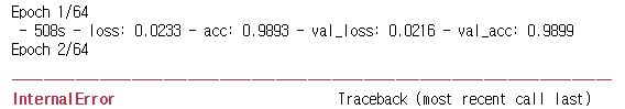
GPU기반 Keras로 코드를 작성하다보면 아래와 같은 오류 메시지에 직면할 때가 있다.

InternalError: Blas GEMM launch failed
CUDA_ERROR_OUT_OF_MEMORY
InternalError: GPU sync failed

GPU에 할당된 메모리를 다른 세션이 점유하고 있어서 발생할 가능성이 높다.
1) 점유하고 있는 세션을 중단하고 메모리를 회수한다.
2) Keras가 사용하는 Backend엔진(ex.Tensorflow)의 메모리 추가 사용을 허락한다.

이 문제를 해결한 후 오류가 발생한 세션을 다시 시작해야한다. 
그렇지 않으면 "InternalError: GPU sync failed"가 발생할 수 있다.


[Tensorflow Backand 엔진 설정 방법]

from keras.backend import tensorflow_backend as K config = tf.ConfigProto() config.gpu_options.allow_growth = True K.set_session(tf.Session(config=config))

전체 소스코드는 아래 포스트를 참고하세요.

[Keras] IRIS데이터 이용한 DNN

IRIS데이터를 이용한 간단한 DNN 학습 및 추론을 해보자. 데이터를 Train/Test로 구분한 후 학습...

blog.naver.com

끝.

--------------------------------------------------------------------------------------

2. https://zereight.tistory.com/228

GPU 동기화 오류이다.

다음 코드를 돌려서 해결하자

import tensorflow as tf

config = tf.ConfigProto()

config.gpu_options.per_process_gpu_memory_fraction = 0.4

session = tf.Session(config=config)

session.close()

--------------------------------------------------------------------------------------

3. https://emmadeveloper.tistory.com/27

GPU sync failed 에러가 떴다.

러닝 시작한 것 확인하고 잤는데 에러 떠 있어서

확인해보니 전용 GPU메모리의 50% 정도를 이미 다른 곳에서 점유하고 있었다.

나머지 것들을 shutdown시켰다.

다시 실행해보려는데 안 됨.

그냥 jupyter notebook을 재실행했더니 다시 잘 된다.

이제 돌리기 전에 전용 GPU 메모리 사용량을 미리 확인하고, 깔끔하게 낮춘 후, 돌려야겠다.

--------------------------------------------------------------------------------------
4. https://stackoverflow.com/questions/51112126/gpu-sync-failed-while-using-tensorflow

TLDR: If you find that tensorflow is throwing a GPU sync failed Error, it may be because the model's inputs are too large (as was my case when first running into this problem) or you don't have cuDNN installed properly. Verify that cuDNN is installed correctly and reset your nvidia caches (ie. sudo -rf $HOME/.nv/) (if you have no yet done so after initially installing CUDA and cuDNN) and restart your machine.

https://machinelearningmastery.com/keras-functional-api-deep-learning/

How to Use the Keras Functional API for Deep Learning

Share on TwitterTweet

Share on Facebook Share

Share on LinkedIn Share

Share on Google Plus Share

The Keras Python library makes creating deep learning models fast and easy.

The sequential API allows you to create models layer-by-layer for most problems. It is limited in that it does not allow you to create models that share layers or have multiple inputs or outputs.

The functional API in Keras is an alternate way of creating models that offers a lot more flexibility, including creating more complex models.

In this tutorial, you will discover how to use the more flexible functional API in Keras to define deep learning models.

After completing this tutorial, you will know:

• The difference between the Sequential and Functional APIs.
• How to define simple Multilayer Perceptron, Convolutional Neural Network, and Recurrent Neural Network models using the functional API.
• How to define more complex models with shared layers and multiple inputs and outputs.

Let’s get started.

Tutorial Overview

This tutorial is divided into 6 parts; they are:

1. Keras Sequential Models
2. Keras Functional Models
3. Standard Network Models
4. Shared Layers Model
5. Multiple Input and Output Models
6. Best Practices

1. Keras Sequential Models

As a review, Keras provides a Sequential model API.

This is a way of creating deep learning models where an instance of the Sequential class is created and model layers are created and added to it.

For example, the layers can be defined and passed to the Sequential as an array:

from keras.models import Sequential from keras.layers import Dense model = Sequential([Dense(2, input_dim=1), Dense(1)])

1 2 3

from keras.models import Sequential from keras.layers import Dense model = Sequential([Dense(2, input_dim=1), Dense(1)])

Layers can also be added piecewise:

from keras.models import Sequential from keras.layers import Dense model = Sequential() model.add(Dense(2, input_dim=1)) model.add(Dense(1))

1 2 3 4 5

from keras.models import Sequential from keras.layers import Dense model = Sequential() model.add(Dense(2, input_dim=1)) model.add(Dense(1))

The Sequential model API is great for developing deep learning models in most situations, but it also has some limitations.

For example, it is not straightforward to define models that may have multiple different input sources, produce multiple output destinations or models that re-use layers.

2. Keras Functional Models

The Keras functional API provides a more flexible way for defining models.

It specifically allows you to define multiple input or output models as well as models that share layers. More than that, it allows you to define ad hoc acyclic network graphs.

Models are defined by creating instances of layers and connecting them directly to each other in pairs, then defining a Model that specifies the layers to act as the input and output to the model.

Let’s look at the three unique aspects of Keras functional API in turn:

1. Defining Input

Unlike the Sequential model, you must create and define a standalone Input layer that specifies the shape of input data.

The input layer takes a shape argument that is a tuple that indicates the dimensionality of the input data.

When input data is one-dimensional, such as for a multilayer Perceptron, the shape must explicitly leave room for the shape of the mini-batch size used when splitting the data when training the network. Therefore, the shape tuple is always defined with a hanging last dimension (2,), for example:

from keras.layers import Input visible = Input(shape=(2,))

1 2	from keras.layers import Input visible = Input(shape=(2,))

 

2. Connecting Layers

The layers in the model are connected pairwise.

This is done by specifying where the input comes from when defining each new layer. A bracket notation is used, such that after the layer is created, the layer from which the input to the current layer comes from is specified.

Let’s make this clear with a short example. We can create the input layer as above, then create a hidden layer as a Dense that receives input only from the input layer.

from keras.layers import Input from keras.layers import Dense visible = Input(shape=(2,)) hidden = Dense(2)(visible)

1 2 3 4

from keras.layers import Input from keras.layers import Dense visible = Input(shape=(2,)) hidden = Dense(2)(visible)

Note the (visible) after the creation of the Dense layer that connects the input layer output as the input to the dense hidden layer.

It is this way of connecting layers piece by piece that gives the functional API its flexibility. For example, you can see how easy it would be to start defining ad hoc graphs of layers.

3. Creating the Model

After creating all of your model layers and connecting them together, you must define the model.

As with the Sequential API, the model is the thing you can summarize, fit, evaluate, and use to make predictions.

Keras provides a Model class that you can use to create a model from your created layers. It requires that you only specify the input and output layers. For example:

from keras.models import Model from keras.layers import Input from keras.layers import Dense visible = Input(shape=(2,)) hidden = Dense(2)(visible) model = Model(inputs=visible, outputs=hidden)

1 2 3 4 5 6

from keras.models import Model from keras.layers import Input from keras.layers import Dense visible = Input(shape=(2,)) hidden = Dense(2)(visible) model = Model(inputs=visible, outputs=hidden)

Now that we know all of the key pieces of the Keras functional API, let’s work through defining a suite of different models and build up some practice with it.

Each example is executable and prints the structure and creates a diagram of the graph. I recommend doing this for your own models to make it clear what exactly you have defined.

My hope is that these examples provide templates for you when you want to define your own models using the functional API in the future.

3. Standard Network Models

When getting started with the functional API, it is a good idea to see how some standard neural network models are defined.

In this section, we will look at defining a simple multilayer Perceptron, convolutional neural network, and recurrent neural network.

These examples will provide a foundation for understanding the more elaborate examples later.

Multilayer Perceptron

In this section, we define a multilayer Perceptron model for binary classification.

The model has 10 inputs, 3 hidden layers with 10, 20, and 10 neurons, and an output layer with 1 output. Rectified linear activation functions are used in each hidden layer and a sigmoid activation function is used in the output layer, for binary classification.

# Multilayer Perceptron from keras.utils import plot_model from keras.models import Model from keras.layers import Input from keras.layers import Dense visible = Input(shape=(10,)) hidden1 = Dense(10, activation='relu')(visible) hidden2 = Dense(20, activation='relu')(hidden1) hidden3 = Dense(10, activation='relu')(hidden2) output = Dense(1, activation='sigmoid')(hidden3) model = Model(inputs=visible, outputs=output) # summarize layers print(model.summary()) # plot graph plot_model(model, to_file='multilayer_perceptron_graph.png')

1 2 3 4 5 6 7 8 9 10 11 12 13 14 15

# Multilayer Perceptron from keras.utils import plot_model from keras.models import Model from keras.layers import Input from keras.layers import Dense visible = Input(shape=(10,)) hidden1 = Dense(10, activation='relu')(visible) hidden2 = Dense(20, activation='relu')(hidden1) hidden3 = Dense(10, activation='relu')(hidden2) output = Dense(1, activation='sigmoid')(hidden3) model = Model(inputs=visible, outputs=output) # summarize layers print(model.summary()) # plot graph plot_model(model, to_file='multilayer_perceptron_graph.png')

Running the example prints the structure of the network.

_________________________________________________________________ Layer (type) Output Shape Param # ================================================================= input_1 (InputLayer) (None, 10) 0 _________________________________________________________________ dense_1 (Dense) (None, 10) 110 _________________________________________________________________ dense_2 (Dense) (None, 20) 220 _________________________________________________________________ dense_3 (Dense) (None, 10) 210 _________________________________________________________________ dense_4 (Dense) (None, 1) 11 ================================================================= Total params: 551 Trainable params: 551 Non-trainable params: 0 _________________________________________________________________

1 2 3 4 5 6 7 8 9 10 11 12 13 14 15 16 17

_________________________________________________________________ Layer (type)                 Output Shape              Param # ================================================================= input_1 (InputLayer)         (None, 10)                0 _________________________________________________________________ dense_1 (Dense)              (None, 10)                110 _________________________________________________________________ dense_2 (Dense)              (None, 20)                220 _________________________________________________________________ dense_3 (Dense)              (None, 10)                210 _________________________________________________________________ dense_4 (Dense)              (None, 1)                 11 ================================================================= Total params: 551 Trainable params: 551 Non-trainable params: 0 _________________________________________________________________

A plot of the model graph is also created and saved to file.

Multilayer Perceptron Network Graph

Convolutional Neural Network

In this section, we will define a convolutional neural network for image classification.

The model receives black and white 64×64 images as input, then has a sequence of two convolutional and pooling layers as feature extractors, followed by a fully connected layer to interpret the features and an output layer with a sigmoid activation for two-class predictions.

# Convolutional Neural Network from keras.utils import plot_model from keras.models import Model from keras.layers import Input from keras.layers import Dense from keras.layers.convolutional import Conv2D from keras.layers.pooling import MaxPooling2D visible = Input(shape=(64,64,1)) conv1 = Conv2D(32, kernel_size=4, activation='relu')(visible) pool1 = MaxPooling2D(pool_size=(2, 2))(conv1) conv2 = Conv2D(16, kernel_size=4, activation='relu')(pool1) pool2 = MaxPooling2D(pool_size=(2, 2))(conv2) hidden1 = Dense(10, activation='relu')(pool2) output = Dense(1, activation='sigmoid')(hidden1) model = Model(inputs=visible, outputs=output) # summarize layers print(model.summary()) # plot graph plot_model(model, to_file='convolutional_neural_network.png')

1 2 3 4 5 6 7 8 9 10 11 12 13 14 15 16 17 18 19

# Convolutional Neural Network from keras.utils import plot_model from keras.models import Model from keras.layers import Input from keras.layers import Dense from keras.layers.convolutional import Conv2D from keras.layers.pooling import MaxPooling2D visible = Input(shape=(64,64,1)) conv1 = Conv2D(32, kernel_size=4, activation='relu')(visible) pool1 = MaxPooling2D(pool_size=(2, 2))(conv1) conv2 = Conv2D(16, kernel_size=4, activation='relu')(pool1) pool2 = MaxPooling2D(pool_size=(2, 2))(conv2) hidden1 = Dense(10, activation='relu')(pool2) output = Dense(1, activation='sigmoid')(hidden1) model = Model(inputs=visible, outputs=output) # summarize layers print(model.summary()) # plot graph plot_model(model, to_file='convolutional_neural_network.png')

Running the example summarizes the model layers.

_________________________________________________________________ Layer (type) Output Shape Param # ================================================================= input_1 (InputLayer) (None, 64, 64, 1) 0 _________________________________________________________________ conv2d_1 (Conv2D) (None, 61, 61, 32) 544 _________________________________________________________________ max_pooling2d_1 (MaxPooling2 (None, 30, 30, 32) 0 _________________________________________________________________ conv2d_2 (Conv2D) (None, 27, 27, 16) 8208 _________________________________________________________________ max_pooling2d_2 (MaxPooling2 (None, 13, 13, 16) 0 _________________________________________________________________ dense_1 (Dense) (None, 13, 13, 10) 170 _________________________________________________________________ dense_2 (Dense) (None, 13, 13, 1) 11 ================================================================= Total params: 8,933 Trainable params: 8,933 Non-trainable params: 0 _________________________________________________________________

1 2 3 4 5 6 7 8 9 10 11 12 13 14 15 16 17 18 19 20 21

_________________________________________________________________ Layer (type)                 Output Shape              Param # ================================================================= input_1 (InputLayer)         (None, 64, 64, 1)         0 _________________________________________________________________ conv2d_1 (Conv2D)            (None, 61, 61, 32)        544 _________________________________________________________________ max_pooling2d_1 (MaxPooling2 (None, 30, 30, 32)        0 _________________________________________________________________ conv2d_2 (Conv2D)            (None, 27, 27, 16)        8208 _________________________________________________________________ max_pooling2d_2 (MaxPooling2 (None, 13, 13, 16)        0 _________________________________________________________________ dense_1 (Dense)              (None, 13, 13, 10)        170 _________________________________________________________________ dense_2 (Dense)              (None, 13, 13, 1)         11 ================================================================= Total params: 8,933 Trainable params: 8,933 Non-trainable params: 0 _________________________________________________________________

A plot of the model graph is also created and saved to file.

Convolutional Neural Network Graph

Recurrent Neural Network

In this section, we will define a long short-term memory recurrent neural network for sequence classification.

The model expects 100 time steps of one feature as input. The model has a single LSTM hidden layer to extract features from the sequence, followed by a fully connected layer to interpret the LSTM output, followed by an output layer for making binary predictions.

# Recurrent Neural Network from keras.utils import plot_model from keras.models import Model from keras.layers import Input from keras.layers import Dense from keras.layers.recurrent import LSTM visible = Input(shape=(100,1)) hidden1 = LSTM(10)(visible) hidden2 = Dense(10, activation='relu')(hidden1) output = Dense(1, activation='sigmoid')(hidden2) model = Model(inputs=visible, outputs=output) # summarize layers print(model.summary()) # plot graph plot_model(model, to_file='recurrent_neural_network.png')

1 2 3 4 5 6 7 8 9 10 11 12 13 14 15

# Recurrent Neural Network from keras.utils import plot_model from keras.models import Model from keras.layers import Input from keras.layers import Dense from keras.layers.recurrent import LSTM visible = Input(shape=(100,1)) hidden1 = LSTM(10)(visible) hidden2 = Dense(10, activation='relu')(hidden1) output = Dense(1, activation='sigmoid')(hidden2) model = Model(inputs=visible, outputs=output) # summarize layers print(model.summary()) # plot graph plot_model(model, to_file='recurrent_neural_network.png')

Running the example summarizes the model layers.

_________________________________________________________________ Layer (type) Output Shape Param # ================================================================= input_1 (InputLayer) (None, 100, 1) 0 _________________________________________________________________ lstm_1 (LSTM) (None, 10) 480 _________________________________________________________________ dense_1 (Dense) (None, 10) 110 _________________________________________________________________ dense_2 (Dense) (None, 1) 11 ================================================================= Total params: 601 Trainable params: 601 Non-trainable params: 0 _________________________________________________________________

1 2 3 4 5 6 7 8 9 10 11 12 13 14 15

_________________________________________________________________ Layer (type)                 Output Shape              Param # ================================================================= input_1 (InputLayer)         (None, 100, 1)            0 _________________________________________________________________ lstm_1 (LSTM)                (None, 10)                480 _________________________________________________________________ dense_1 (Dense)              (None, 10)                110 _________________________________________________________________ dense_2 (Dense)              (None, 1)                 11 ================================================================= Total params: 601 Trainable params: 601 Non-trainable params: 0 _________________________________________________________________

A plot of the model graph is also created and saved to file.

Recurrent Neural Network Graph

4. Shared Layers Model

Multiple layers can share the output from one layer.

For example, there may be multiple different feature extraction layers from an input, or multiple layers used to interpret the output from a feature extraction layer.

Let’s look at both of these examples.

Shared Input Layer

In this section, we define multiple convolutional layers with differently sized kernels to interpret an image input.

The model takes black and white images with the size 64×64 pixels. There are two CNN feature extraction submodels that share this input; the first has a kernel size of 4 and the second a kernel size of 8. The outputs from these feature extraction submodels are flattened into vectors and concatenated into one long vector and passed on to a fully connected layer for interpretation before a final output layer makes a binary classification.

# Shared Input Layer from keras.utils import plot_model from keras.models import Model from keras.layers import Input from keras.layers import Dense from keras.layers import Flatten from keras.layers.convolutional import Conv2D from keras.layers.pooling import MaxPooling2D from keras.layers.merge import concatenate # input layer visible = Input(shape=(64,64,1)) # first feature extractor conv1 = Conv2D(32, kernel_size=4, activation='relu')(visible) pool1 = MaxPooling2D(pool_size=(2, 2))(conv1) flat1 = Flatten()(pool1) # second feature extractor conv2 = Conv2D(16, kernel_size=8, activation='relu')(visible) pool2 = MaxPooling2D(pool_size=(2, 2))(conv2) flat2 = Flatten()(pool2) # merge feature extractors merge = concatenate([flat1, flat2]) # interpretation layer hidden1 = Dense(10, activation='relu')(merge) # prediction output output = Dense(1, activation='sigmoid')(hidden1) model = Model(inputs=visible, outputs=output) # summarize layers print(model.summary()) # plot graph plot_model(model, to_file='shared_input_layer.png')

1 2 3 4 5 6 7 8 9 10 11 12 13 14 15 16 17 18 19 20 21 22 23 24 25 26 27 28 29 30

# Shared Input Layer from keras.utils import plot_model from keras.models import Model from keras.layers import Input from keras.layers import Dense from keras.layers import Flatten from keras.layers.convolutional import Conv2D from keras.layers.pooling import MaxPooling2D from keras.layers.merge import concatenate # input layer visible = Input(shape=(64,64,1)) # first feature extractor conv1 = Conv2D(32, kernel_size=4, activation='relu')(visible) pool1 = MaxPooling2D(pool_size=(2, 2))(conv1) flat1 = Flatten()(pool1) # second feature extractor conv2 = Conv2D(16, kernel_size=8, activation='relu')(visible) pool2 = MaxPooling2D(pool_size=(2, 2))(conv2) flat2 = Flatten()(pool2) # merge feature extractors merge = concatenate([flat1, flat2]) # interpretation layer hidden1 = Dense(10, activation='relu')(merge) # prediction output output = Dense(1, activation='sigmoid')(hidden1) model = Model(inputs=visible, outputs=output) # summarize layers print(model.summary()) # plot graph plot_model(model, to_file='shared_input_layer.png')

Running the example summarizes the model layers.

____________________________________________________________________________________________________ Layer (type) Output Shape Param # Connected to ==================================================================================================== input_1 (InputLayer) (None, 64, 64, 1) 0 ____________________________________________________________________________________________________ conv2d_1 (Conv2D) (None, 61, 61, 32) 544 input_1[0][0] ____________________________________________________________________________________________________ conv2d_2 (Conv2D) (None, 57, 57, 16) 1040 input_1[0][0] ____________________________________________________________________________________________________ max_pooling2d_1 (MaxPooling2D) (None, 30, 30, 32) 0 conv2d_1[0][0] ____________________________________________________________________________________________________ max_pooling2d_2 (MaxPooling2D) (None, 28, 28, 16) 0 conv2d_2[0][0] ____________________________________________________________________________________________________ flatten_1 (Flatten) (None, 28800) 0 max_pooling2d_1[0][0] ____________________________________________________________________________________________________ flatten_2 (Flatten) (None, 12544) 0 max_pooling2d_2[0][0] ____________________________________________________________________________________________________ concatenate_1 (Concatenate) (None, 41344) 0 flatten_1[0][0] flatten_2[0][0] ____________________________________________________________________________________________________ dense_1 (Dense) (None, 10) 413450 concatenate_1[0][0] ____________________________________________________________________________________________________ dense_2 (Dense) (None, 1) 11 dense_1[0][0] ==================================================================================================== Total params: 415,045 Trainable params: 415,045 Non-trainable params: 0 ____________________________________________________________________________________________________

1 2 3 4 5 6 7 8 9 10 11 12 13 14 15 16 17 18 19 20 21 22 23 24 25 26 27 28

____________________________________________________________________________________________________ Layer (type)                     Output Shape          Param #     Connected to ==================================================================================================== input_1 (InputLayer)             (None, 64, 64, 1)     0 ____________________________________________________________________________________________________ conv2d_1 (Conv2D)                (None, 61, 61, 32)    544         input_1[0][0] ____________________________________________________________________________________________________ conv2d_2 (Conv2D)                (None, 57, 57, 16)    1040        input_1[0][0] ____________________________________________________________________________________________________ max_pooling2d_1 (MaxPooling2D)   (None, 30, 30, 32)    0           conv2d_1[0][0] ____________________________________________________________________________________________________ max_pooling2d_2 (MaxPooling2D)   (None, 28, 28, 16)    0           conv2d_2[0][0] ____________________________________________________________________________________________________ flatten_1 (Flatten)              (None, 28800)         0           max_pooling2d_1[0][0] ____________________________________________________________________________________________________ flatten_2 (Flatten)              (None, 12544)         0           max_pooling2d_2[0][0] ____________________________________________________________________________________________________ concatenate_1 (Concatenate)      (None, 41344)         0           flatten_1[0][0]                                                                    flatten_2[0][0] ____________________________________________________________________________________________________ dense_1 (Dense)                  (None, 10)            413450      concatenate_1[0][0] ____________________________________________________________________________________________________ dense_2 (Dense)                  (None, 1)             11          dense_1[0][0] ==================================================================================================== Total params: 415,045 Trainable params: 415,045 Non-trainable params: 0 ____________________________________________________________________________________________________

A plot of the model graph is also created and saved to file.

Neural Network Graph With Shared Inputs

Shared Feature Extraction Layer

In this section, we will two parallel submodels to interpret the output of an LSTM feature extractor for sequence classification.

The input to the model is 100 time steps of 1 feature. An LSTM layer with 10 memory cells interprets this sequence. The first interpretation model is a shallow single fully connected layer, the second is a deep 3 layer model. The output of both interpretation models are concatenated into one long vector that is passed to the output layer used to make a binary prediction.

# Shared Feature Extraction Layer from keras.utils import plot_model from keras.models import Model from keras.layers import Input from keras.layers import Dense from keras.layers.recurrent import LSTM from keras.layers.merge import concatenate # define input visible = Input(shape=(100,1)) # feature extraction extract1 = LSTM(10)(visible) # first interpretation model interp1 = Dense(10, activation='relu')(extract1) # second interpretation model interp11 = Dense(10, activation='relu')(extract1) interp12 = Dense(20, activation='relu')(interp11) interp13 = Dense(10, activation='relu')(interp12) # merge interpretation merge = concatenate([interp1, interp13]) # output output = Dense(1, activation='sigmoid')(merge) model = Model(inputs=visible, outputs=output) # summarize layers print(model.summary()) # plot graph plot_model(model, to_file='shared_feature_extractor.png')

1 2 3 4 5 6 7 8 9 10 11 12 13 14 15 16 17 18 19 20 21 22 23 24 25 26

# Shared Feature Extraction Layer from keras.utils import plot_model from keras.models import Model from keras.layers import Input from keras.layers import Dense from keras.layers.recurrent import LSTM from keras.layers.merge import concatenate # define input visible = Input(shape=(100,1)) # feature extraction extract1 = LSTM(10)(visible) # first interpretation model interp1 = Dense(10, activation='relu')(extract1) # second interpretation model interp11 = Dense(10, activation='relu')(extract1) interp12 = Dense(20, activation='relu')(interp11) interp13 = Dense(10, activation='relu')(interp12) # merge interpretation merge = concatenate([interp1, interp13]) # output output = Dense(1, activation='sigmoid')(merge) model = Model(inputs=visible, outputs=output) # summarize layers print(model.summary()) # plot graph plot_model(model, to_file='shared_feature_extractor.png')

Running the example summarizes the model layers.

____________________________________________________________________________________________________ Layer (type) Output Shape Param # Connected to ==================================================================================================== input_1 (InputLayer) (None, 100, 1) 0 ____________________________________________________________________________________________________ lstm_1 (LSTM) (None, 10) 480 input_1[0][0] ____________________________________________________________________________________________________ dense_2 (Dense) (None, 10) 110 lstm_1[0][0] ____________________________________________________________________________________________________ dense_3 (Dense) (None, 20) 220 dense_2[0][0] ____________________________________________________________________________________________________ dense_1 (Dense) (None, 10) 110 lstm_1[0][0] ____________________________________________________________________________________________________ dense_4 (Dense) (None, 10) 210 dense_3[0][0] ____________________________________________________________________________________________________ concatenate_1 (Concatenate) (None, 20) 0 dense_1[0][0] dense_4[0][0] ____________________________________________________________________________________________________ dense_5 (Dense) (None, 1) 21 concatenate_1[0][0] ==================================================================================================== Total params: 1,151 Trainable params: 1,151 Non-trainable params: 0 ____________________________________________________________________________________________________

1 2 3 4 5 6 7 8 9 10 11 12 13 14 15 16 17 18 19 20 21 22 23 24

____________________________________________________________________________________________________ Layer (type)                     Output Shape          Param #     Connected to ==================================================================================================== input_1 (InputLayer)             (None, 100, 1)        0 ____________________________________________________________________________________________________ lstm_1 (LSTM)                    (None, 10)            480         input_1[0][0] ____________________________________________________________________________________________________ dense_2 (Dense)                  (None, 10)            110         lstm_1[0][0] ____________________________________________________________________________________________________ dense_3 (Dense)                  (None, 20)            220         dense_2[0][0] ____________________________________________________________________________________________________ dense_1 (Dense)                  (None, 10)            110         lstm_1[0][0] ____________________________________________________________________________________________________ dense_4 (Dense)                  (None, 10)            210         dense_3[0][0] ____________________________________________________________________________________________________ concatenate_1 (Concatenate)      (None, 20)            0           dense_1[0][0]                                                                    dense_4[0][0] ____________________________________________________________________________________________________ dense_5 (Dense)                  (None, 1)             21          concatenate_1[0][0] ==================================================================================================== Total params: 1,151 Trainable params: 1,151 Non-trainable params: 0 ____________________________________________________________________________________________________

A plot of the model graph is also created and saved to file.

Neural Network Graph With Shared Feature Extraction Layer

5. Multiple Input and Output Models

The functional API can also be used to develop more complex models with multiple inputs, possibly with different modalities. It can also be used to develop models that produce multiple outputs.

We will look at examples of each in this section.

Multiple Input Model

We will develop an image classification model that takes two versions of the image as input, each of a different size. Specifically a black and white 64×64 version and a color 32×32 version. Separate feature extraction CNN models operate on each, then the results from both models are concatenated for interpretation and ultimate prediction.

Note that in the creation of the Model() instance, that we define the two input layers as an array. Specifically:

model = Model(inputs=[visible1, visible2], outputs=output)

1	model = Model(inputs=[visible1, visible2], outputs=output)

The complete example is listed below.

# Multiple Inputs from keras.utils import plot_model from keras.models import Model from keras.layers import Input from keras.layers import Dense from keras.layers import Flatten from keras.layers.convolutional import Conv2D from keras.layers.pooling import MaxPooling2D from keras.layers.merge import concatenate # first input model visible1 = Input(shape=(64,64,1)) conv11 = Conv2D(32, kernel_size=4, activation='relu')(visible1) pool11 = MaxPooling2D(pool_size=(2, 2))(conv11) conv12 = Conv2D(16, kernel_size=4, activation='relu')(pool11) pool12 = MaxPooling2D(pool_size=(2, 2))(conv12) flat1 = Flatten()(pool12) # second input model visible2 = Input(shape=(32,32,3)) conv21 = Conv2D(32, kernel_size=4, activation='relu')(visible2) pool21 = MaxPooling2D(pool_size=(2, 2))(conv21) conv22 = Conv2D(16, kernel_size=4, activation='relu')(pool21) pool22 = MaxPooling2D(pool_size=(2, 2))(conv22) flat2 = Flatten()(pool22) # merge input models merge = concatenate([flat1, flat2]) # interpretation model hidden1 = Dense(10, activation='relu')(merge) hidden2 = Dense(10, activation='relu')(hidden1) output = Dense(1, activation='sigmoid')(hidden2) model = Model(inputs=[visible1, visible2], outputs=output) # summarize layers print(model.summary()) # plot graph plot_model(model, to_file='multiple_inputs.png')

1 2 3 4 5 6 7 8 9 10 11 12 13 14 15 16 17 18 19 20 21 22 23 24 25 26 27 28 29 30 31 32 33 34

# Multiple Inputs from keras.utils import plot_model from keras.models import Model from keras.layers import Input from keras.layers import Dense from keras.layers import Flatten from keras.layers.convolutional import Conv2D from keras.layers.pooling import MaxPooling2D from keras.layers.merge import concatenate # first input model visible1 = Input(shape=(64,64,1)) conv11 = Conv2D(32, kernel_size=4, activation='relu')(visible1) pool11 = MaxPooling2D(pool_size=(2, 2))(conv11) conv12 = Conv2D(16, kernel_size=4, activation='relu')(pool11) pool12 = MaxPooling2D(pool_size=(2, 2))(conv12) flat1 = Flatten()(pool12) # second input model visible2 = Input(shape=(32,32,3)) conv21 = Conv2D(32, kernel_size=4, activation='relu')(visible2) pool21 = MaxPooling2D(pool_size=(2, 2))(conv21) conv22 = Conv2D(16, kernel_size=4, activation='relu')(pool21) pool22 = MaxPooling2D(pool_size=(2, 2))(conv22) flat2 = Flatten()(pool22) # merge input models merge = concatenate([flat1, flat2]) # interpretation model hidden1 = Dense(10, activation='relu')(merge) hidden2 = Dense(10, activation='relu')(hidden1) output = Dense(1, activation='sigmoid')(hidden2) model = Model(inputs=[visible1, visible2], outputs=output) # summarize layers print(model.summary()) # plot graph plot_model(model, to_file='multiple_inputs.png')

Running the example summarizes the model layers.

____________________________________________________________________________________________________ Layer (type) Output Shape Param # Connected to ==================================================================================================== input_1 (InputLayer) (None, 64, 64, 1) 0 ____________________________________________________________________________________________________ input_2 (InputLayer) (None, 32, 32, 3) 0 ____________________________________________________________________________________________________ conv2d_1 (Conv2D) (None, 61, 61, 32) 544 input_1[0][0] ____________________________________________________________________________________________________ conv2d_3 (Conv2D) (None, 29, 29, 32) 1568 input_2[0][0] ____________________________________________________________________________________________________ max_pooling2d_1 (MaxPooling2D) (None, 30, 30, 32) 0 conv2d_1[0][0] ____________________________________________________________________________________________________ max_pooling2d_3 (MaxPooling2D) (None, 14, 14, 32) 0 conv2d_3[0][0] ____________________________________________________________________________________________________ conv2d_2 (Conv2D) (None, 27, 27, 16) 8208 max_pooling2d_1[0][0] ____________________________________________________________________________________________________ conv2d_4 (Conv2D) (None, 11, 11, 16) 8208 max_pooling2d_3[0][0] ____________________________________________________________________________________________________ max_pooling2d_2 (MaxPooling2D) (None, 13, 13, 16) 0 conv2d_2[0][0] ____________________________________________________________________________________________________ max_pooling2d_4 (MaxPooling2D) (None, 5, 5, 16) 0 conv2d_4[0][0] ____________________________________________________________________________________________________ flatten_1 (Flatten) (None, 2704) 0 max_pooling2d_2[0][0] ____________________________________________________________________________________________________ flatten_2 (Flatten) (None, 400) 0 max_pooling2d_4[0][0] ____________________________________________________________________________________________________ concatenate_1 (Concatenate) (None, 3104) 0 flatten_1[0][0] flatten_2[0][0] ____________________________________________________________________________________________________ dense_1 (Dense) (None, 10) 31050 concatenate_1[0][0] ____________________________________________________________________________________________________ dense_2 (Dense) (None, 10) 110 dense_1[0][0] ____________________________________________________________________________________________________ dense_3 (Dense) (None, 1) 11 dense_2[0][0] ==================================================================================================== Total params: 49,699 Trainable params: 49,699 Non-trainable params: 0 ____________________________________________________________________________________________________

1 2 3 4 5 6 7 8 9 10 11 12 13 14 15 16 17 18 19 20 21 22 23 24 25 26 27 28 29 30 31 32 33 34 35 36 37 38 39 40

____________________________________________________________________________________________________ Layer (type)                     Output Shape          Param #     Connected to ==================================================================================================== input_1 (InputLayer)             (None, 64, 64, 1)     0 ____________________________________________________________________________________________________ input_2 (InputLayer)             (None, 32, 32, 3)     0 ____________________________________________________________________________________________________ conv2d_1 (Conv2D)                (None, 61, 61, 32)    544         input_1[0][0] ____________________________________________________________________________________________________ conv2d_3 (Conv2D)                (None, 29, 29, 32)    1568        input_2[0][0] ____________________________________________________________________________________________________ max_pooling2d_1 (MaxPooling2D)   (None, 30, 30, 32)    0           conv2d_1[0][0] ____________________________________________________________________________________________________ max_pooling2d_3 (MaxPooling2D)   (None, 14, 14, 32)    0           conv2d_3[0][0] ____________________________________________________________________________________________________ conv2d_2 (Conv2D)                (None, 27, 27, 16)    8208        max_pooling2d_1[0][0] ____________________________________________________________________________________________________ conv2d_4 (Conv2D)                (None, 11, 11, 16)    8208        max_pooling2d_3[0][0] ____________________________________________________________________________________________________ max_pooling2d_2 (MaxPooling2D)   (None, 13, 13, 16)    0           conv2d_2[0][0] ____________________________________________________________________________________________________ max_pooling2d_4 (MaxPooling2D)   (None, 5, 5, 16)      0           conv2d_4[0][0] ____________________________________________________________________________________________________ flatten_1 (Flatten)              (None, 2704)          0           max_pooling2d_2[0][0] ____________________________________________________________________________________________________ flatten_2 (Flatten)              (None, 400)           0           max_pooling2d_4[0][0] ____________________________________________________________________________________________________ concatenate_1 (Concatenate)      (None, 3104)          0           flatten_1[0][0]                                                                    flatten_2[0][0] ____________________________________________________________________________________________________ dense_1 (Dense)                  (None, 10)            31050       concatenate_1[0][0] ____________________________________________________________________________________________________ dense_2 (Dense)                  (None, 10)            110         dense_1[0][0] ____________________________________________________________________________________________________ dense_3 (Dense)                  (None, 1)             11          dense_2[0][0] ==================================================================================================== Total params: 49,699 Trainable params: 49,699 Non-trainable params: 0 ____________________________________________________________________________________________________

A plot of the model graph is also created and saved to file.

Neural Network Graph With Multiple Inputs

Multiple Output Model

In this section, we will develop a model that makes two different types of predictions. Given an input sequence of 100 time steps of one feature, the model will both classify the sequence and output a new sequence with the same length.

An LSTM layer interprets the input sequence and returns the hidden state for each time step. The first output model creates a stacked LSTM, interprets the features, and makes a binary prediction. The second output model uses the same output layer to make a real-valued prediction for each input time step.

# Multiple Outputs from keras.utils import plot_model from keras.models import Model from keras.layers import Input from keras.layers import Dense from keras.layers.recurrent import LSTM from keras.layers.wrappers import TimeDistributed # input layer visible = Input(shape=(100,1)) # feature extraction extract = LSTM(10, return_sequences=True)(visible) # classification output class11 = LSTM(10)(extract) class12 = Dense(10, activation='relu')(class11) output1 = Dense(1, activation='sigmoid')(class12) # sequence output output2 = TimeDistributed(Dense(1, activation='linear'))(extract) # output model = Model(inputs=visible, outputs=[output1, output2]) # summarize layers print(model.summary()) # plot graph plot_model(model, to_file='multiple_outputs.png')

1 2 3 4 5 6 7 8 9 10 11 12 13 14 15 16 17 18 19 20 21 22 23

# Multiple Outputs from keras.utils import plot_model from keras.models import Model from keras.layers import Input from keras.layers import Dense from keras.layers.recurrent import LSTM from keras.layers.wrappers import TimeDistributed # input layer visible = Input(shape=(100,1)) # feature extraction extract = LSTM(10, return_sequences=True)(visible) # classification output class11 = LSTM(10)(extract) class12 = Dense(10, activation='relu')(class11) output1 = Dense(1, activation='sigmoid')(class12) # sequence output output2 = TimeDistributed(Dense(1, activation='linear'))(extract) # output model = Model(inputs=visible, outputs=[output1, output2]) # summarize layers print(model.summary()) # plot graph plot_model(model, to_file='multiple_outputs.png')

Running the example summarizes the model layers.

____________________________________________________________________________________________________ Layer (type) Output Shape Param # Connected to ==================================================================================================== input_1 (InputLayer) (None, 100, 1) 0 ____________________________________________________________________________________________________ lstm_1 (LSTM) (None, 100, 10) 480 input_1[0][0] ____________________________________________________________________________________________________ lstm_2 (LSTM) (None, 10) 840 lstm_1[0][0] ____________________________________________________________________________________________________ dense_1 (Dense) (None, 10) 110 lstm_2[0][0] ____________________________________________________________________________________________________ dense_2 (Dense) (None, 1) 11 dense_1[0][0] ____________________________________________________________________________________________________ time_distributed_1 (TimeDistribu (None, 100, 1) 11 lstm_1[0][0] ==================================================================================================== Total params: 1,452 Trainable params: 1,452 Non-trainable params: 0 ____________________________________________________________________________________________________

1 2 3 4 5 6 7 8 9 10 11 12 13 14 15 16 17 18 19

____________________________________________________________________________________________________ Layer (type)                     Output Shape          Param #     Connected to ==================================================================================================== input_1 (InputLayer)             (None, 100, 1)        0 ____________________________________________________________________________________________________ lstm_1 (LSTM)                    (None, 100, 10)       480         input_1[0][0] ____________________________________________________________________________________________________ lstm_2 (LSTM)                    (None, 10)            840         lstm_1[0][0] ____________________________________________________________________________________________________ dense_1 (Dense)                  (None, 10)            110         lstm_2[0][0] ____________________________________________________________________________________________________ dense_2 (Dense)                  (None, 1)             11          dense_1[0][0] ____________________________________________________________________________________________________ time_distributed_1 (TimeDistribu (None, 100, 1)        11          lstm_1[0][0] ==================================================================================================== Total params: 1,452 Trainable params: 1,452 Non-trainable params: 0 ____________________________________________________________________________________________________

A plot of the model graph is also created and saved to file.

Neural Network Graph With Multiple Outputs

6. Best Practices

In this section, I want to give you some tips to get the most out of the functional API when you are defining your own models.

• Consistent Variable Names. Use the same variable name for the input (visible) and output layers (output) and perhaps even the hidden layers (hidden1, hidden2). It will help to connect things together correctly.
• Review Layer Summary. Always print the model summary and review the layer outputs to ensure that the model was connected together as you expected.
• Review Graph Plots. Always create a plot of the model graph and review it to ensure that everything was put together as you intended.
• Name the layers. You can assign names to layers that are used when reviewing summaries and plots of the model graph. For example: Dense(1, name=’hidden1′).
• Separate Submodels. Consider separating out the development of submodels and combine the submodels together at the end.

Do you have your own best practice tips when using the functional API?
Let me know in the comments.

Further Reading

This section provides more resources on the topic if you are looking go deeper.

• The Sequential model API
• Getting started with the Keras Sequential model
• Getting started with the Keras functional API
• Model class Functional API

Summary

In this tutorial, you discovered how to use the functional API in Keras for defining simple and complex deep learning models.

Specifically, you learned:

• The difference between the Sequential and Functional APIs.
• How to define simple Multilayer Perceptron, Convolutional Neural Network, and Recurrent Neural Network models using the functional API.
• How to define more complex models with shared layers and multiple inputs and outputs.

Do you have any questions?
Ask your questions in the comments below and I will do my best to answer.

https://www.facebook.com/nextobe1/posts/341026106333391

LSTM을 이용한 감정 분석 w/ Tensorflow
O'Reilly의 서버에서 미리 빌드된 환경에서 이 코드를 셀 단위로 실행하거나 자신의 컴퓨터에서 이 파일을 실행할 수 있습니다. 또한 사전 에 Pre-Trained LSTM.ipynb로 자신 만의 텍스트를 입력하고 훈련된 네트워크의 출력을 볼 수 있습니다.

깃허브
https://github.com/adeshpande3/LSTM-Sentiment-Analysis

Google’s TensorFlow has been a hot topic in deep learning recently.  The open source software, designed to allow efficient computation of data flow graphs, is especially suited to deep learning tasks.  It is designed to be executed on single or multiple CPUs and GPUs, making it a good option for complex deep learning tasks.  In it’s most recent incarnation – version 1.0 – it can even be run on certain mobile operating systems.

This introductory tutorial to TensorFlow will give an overview of some of the basic concepts of TensorFlow in Python.  These will be a good stepping stone to building more complex deep learning networks, such as Convolution Neural Networks and Recurrent Neural Networks, in the package.  We’ll be creating a simple three-layer neural network to classify the MNIST dataset.  This tutorial assumes that you are familiar with the basics of neural networks, which you can get up to scratch with in the neural networks tutorial if required.  To install TensorFlow, follow the instructions here. First, let’s have a look at the main ideas of TensorFlow.

1.0 TensorFlow graphs

TensorFlow is based on graph based computation – “what on earth is that?”, you might say.  It’s an alternative way of conceptualising mathematical calculations.  Consider the following expression a=(b+c)∗(c+2) $a=(b+c)\ast (c+2)$ .  We can break this function down into the following components:

Now we can represent these operations graphically as:

This may seem like a silly example – but notice a powerful idea in expressing the equation this way: two of the computations (d=b+c $d=b+c$ and e=c+2 $e=c+2$ ) can be performed in parallel.  By splitting up these calculations across CPUs or GPUs, this can give us significant gains in computational times.  These gains are a must for big data applications and deep learning – especially for complicated neural network architectures such as Convolutional Neural Networks (CNNs) and Recurrent Neural Networks (RNNs).  The idea behind TensorFlow is to ability to create these computational graphs in code and allow significant performance improvements via parallel operations and other efficiency gains.

We can look at a similar graph in TensorFlow below, which shows the computational graph of a three-layer neural network.

The animated data flows between different nodes in the graph are tensors which are multi-dimensional data arrays.  For instance, the input data tensor may be 5000 x 64 x 1, which represents a 64 node input layer with 5000 training samples.  After the input layer there is a hidden layer with rectified linear units as the activation function.  There is a final output layer (called a “logit layer” in the above graph) which uses cross entropy as a cost/loss function.  At each point we see the relevant tensors flowing to the “Gradients” block which finally flow to the Stochastic Gradient Descent optimiser which performs the back-propagation and gradient descent.

Here we can see how computational graphs can be used to represent the calculations in neural networks, and this, of course, is what TensorFlow excels at.  Let’s see how to perform some basic mathematical operations in TensorFlow to get a feel for how it all works.

2.0 A Simple TensorFlow example

Let’s first make TensorFlow perform our little example calculation above – a=(b+c)∗(c+2) $a=(b+c)\ast (c+2)$ .  First we need to introduce ourselves to TensorFlow variables and constants.  Let’s declare some then I’ll explain the syntax:

import tensorflow as tf

# first, create a TensorFlow constant
const = tf.constant(2.0, name="const")
    
# create TensorFlow variables
b = tf.Variable(2.0, name='b')
c = tf.Variable(1.0, name='c')

As can be observed above, TensorFlow constants can be declared using the tf.constant function, and variables with the tf.Variable function.  The first element in both is the value to be assigned the constant / variable when it is initialised.  The second is an optional name string which can be used to label the constant / variable – this is handy for when you want to do visualisations (as will be discussed briefly later).  TensorFlow will infer the type of the constant / variable from the initialised value, but it can also be set explicitly using the optional dtype argument.  TensorFlow has many of its own types like tf.float32, tf.int32 etc. – see them all here.

It’s important to note that, as the Python code runs through these commands, the variables haven’t actually been declared as they would have been if you just had a standard Python declaration (i.e. b = 2.0).  Instead, all the constants, variables, operations and the computational graph are only created when the initialisation commands are run.

Next, we create the TensorFlow operations:

# now create some operations
d = tf.add(b, c, name='d')
e = tf.add(c, const, name='e')
a = tf.multiply(d, e, name='a')

TensorFlow has a wealth of operations available to perform all sorts of interactions between variables, some of which we’ll get to later in the tutorial.  The operations above are pretty obvious, and they instantiate the operations b+c $b+c$ , c+2.0 $c+2.0$ and d∗e $d\ast e$ .

The next step is to setup an object to initialise the variables and the graph structure:

# setup the variable initialisation
init_op = tf.global_variables_initializer()

Ok, so now we are all set to go.  To run the operations between the variables, we need to start a TensorFlow session – tf.Session.  The TensorFlow session is an object where all operations are run.  Using the with Python syntax, we can run the graph with the following code:

# start the session
with tf.Session() as sess:
    # initialise the variables
    sess.run(init_op)
    # compute the output of the graph
    a_out = sess.run(a)
    print("Variable a is {}".format(a_out))

The first command within the with block is the initialisation, which is run with the, well, run command.  Next we want to figure out what the variable a should be.  All we have to do is run the operation which calculates a i.e. a = tf.multiply(d, e, name=’a’).  Note that a is an operation, not a variable and therefore it can be run.  We do just that with the sess.run(a) command and assign the output to a_out, the value of which we then print out.

Note something cool – we defined operations d and e which need to be calculated before we can figure out what a is.  However, we don’t have to explicitly run those operations, as TensorFlow knows what other operations and variables the operation a depends on, and therefore runs the necessary operations on its own.  It does this through its data flow graph which shows it all the required dependencies. Using the TensorBoard functionality, we can see the graph that TensorFlow created in this little program:

Now that’s obviously a trivial example – what if we had an array of b values that we wanted to calculate the value of a over?

2.1 The TensorFlow placeholder

Let’s also say that we didn’t know what the value of the array b would be during the declaration phase of the TensorFlow problem (i.e. before the with tf.Session() as sess) stage.  In this case, TensorFlow requires us to declare the basic structure of the data by using the tf.placeholder variable declaration.  Let’s use it for b:

# create TensorFlow variables
b = tf.placeholder(tf.float32, [None, 1], name='b')

Because we aren’t providing an initialisation in this declaration, we need to tell TensorFlow what data type each element within the tensor is going to be.  In this case, we want to use tf.float32.  The second argument is the shape of the data that will be “injected” into this variable.  In this case, we want to use a (? x 1) sized array – because we are being cagey about how much data we are supplying to this variable (hence the “?”), the placeholder is willing to accept a None argument in the size declaration.  Now we can inject as much 1-dimensional data that we want into the b variable.

The only other change we need to make to our program is in the sess.run(a,…) command:

a_out = sess.run(a, feed_dict={b: np.arange(0, 10)[:, np.newaxis]})

Note that we have added the feed_dict argument to the sess.run(a,…) command.  Here we remove the mystery and specify exactly what the variable b is to be – a one-dimensional range from 0 to 10.  As suggested by the argument name, feed_dict, the input to be supplied is a Python dictionary, with each key being the name of the placeholder that we are filling.

When we run the program again this time we get:

Variable a is [[  3.]
 [  6.]
 [  9.]
 [ 12.]
 [ 15.]
 [ 18.]
 [ 21.]
 [ 24.]
 [ 27.]
 [ 30.]]

Notice how TensorFlow adapts naturally from a scalar output (i.e. a singular output when a=9.0) to a tensor (i.e. an array/matrix)?  This is based on its understanding of how the data will flow through the graph.

Now we are ready to build a basic MNIST predicting neural network.

3.0 A Neural Network Example

Now we’ll go through an example in TensorFlow of creating a simple three layer neural network.  In future articles, we’ll show how to build more complicated neural network structures such as convolution neural networks and recurrent neural networks.  For this example though, we’ll keep it simple.  If you need to scrub up on your neural network basics, check out my popular tutorial on the subject.  In this example, we’ll be using the MNIST dataset (and its associated loader) that the TensorFlow package provides.  This MNIST dataset is a set of 28×28 pixel grayscale images which represent hand-written digits.  It has 55,000 training rows, 10,000 testing rows and 5,000 validation rows.

We can load the data by running:

from tensorflow.examples.tutorials.mnist import input_data
mnist = input_data.read_data_sets("MNIST_data/", one_hot=True)

The one_hot=True argument specifies that instead of the labels associated with each image being the digit itself i.e. “4”, it is a vector with “one hot” node and all the other nodes being zero i.e. [0, 0, 0, 0, 1, 0, 0, 0, 0, 0].  This lets us easily feed it into the output layer of our neural network.

3.1 Setting things up

Next, we can set-up the placeholder variables for the training data (and some training parameters):

# Python optimisation variables
learning_rate = 0.5
epochs = 10
batch_size = 100

# declare the training data placeholders
# input x - for 28 x 28 pixels = 784
x = tf.placeholder(tf.float32, [None, 784])
# now declare the output data placeholder - 10 digits
y = tf.placeholder(tf.float32, [None, 10])

Notice the x input layer is 784 nodes corresponding to the 28 x 28 (=784) pixels, and the y output layer is 10 nodes corresponding to the 10 possible digits.  Again, the size of x is (? x 784), where the ? stands for an as yet unspecified number of samples to be input – this is the function of the placeholder variable.

Now we need to setup the weight and bias variables for the three layer neural network.  There are always L-1 number of weights/bias tensors, where L is the number of layers.  So in this case, we need to setup two tensors for each:

# now declare the weights connecting the input to the hidden layer
W1 = tf.Variable(tf.random_normal([784, 300], stddev=0.03), name='W1')
b1 = tf.Variable(tf.random_normal([300]), name='b1')
# and the weights connecting the hidden layer to the output layer
W2 = tf.Variable(tf.random_normal([300, 10], stddev=0.03), name='W2')
b2 = tf.Variable(tf.random_normal([10]), name='b2')

Ok, so let’s unpack the above code a little.  First, we declare some variables for W1 and b1, the weights and bias for the connections between the input and hidden layer.  This neural network will have 300 nodes in the hidden layer, so the size of the weight tensor W1 is [784, 300].  We initialise the values of the weights using a random normal distribution with a mean of zero and a standard deviation of 0.03.  TensorFlow has a replicated version of the numpy random normal function, which allows you to create a matrix of a given size populated with random samples drawn from a given distribution.  Likewise, we create W2 and b2 variables to connect the hidden layer to the output layer of the neural network.

Next, we have to setup node inputs and activation functions of the hidden layer nodes:

# calculate the output of the hidden layer
hidden_out = tf.add(tf.matmul(x, W1), b1)
hidden_out = tf.nn.relu(hidden_out)

In the first line, we execute the standard matrix multiplication of the weights (W1) by the input vector x and we add the bias b1.  The matrix multiplication is executed using the tf.matmul operation.  Next, we finalise the hidden_out operation by applying a rectified linear unit activation function to the matrix multiplication plus bias.  Note that TensorFlow has a rectified linear unit activation already setup for us, tf.nn.relu.

This is to execute the following equations, as detailed in the neural networks tutorial:

Now, let’s setup the output layer, y_:

# now calculate the hidden layer output - in this case, let's use a softmax activated
# output layer
y_ = tf.nn.softmax(tf.add(tf.matmul(hidden_out, W2), b2))

Again we perform the weight multiplication with the output from the hidden layer (hidden_out) and add the bias, b2.  In this case, we are going to use a softmax activation for the output layer – we can use the included TensorFlow softmax function tf.nn.softmax.

We also have to include a cost or loss function for the optimisation / backpropagation to work on. Here we’ll use the cross entropy cost function, represented by:

Where y (i) j  $y_j^{(i)}$ is the ith training label for output node j, y j _ (i)  $y_j{\mathrm{\_}}^{(i)}$ is the ith predicted label for output node j, m is the number of training / batch samples and n is the number .  There are two operations occurring in the above equation.  The first is the summation of the logarithmic products and additions across all the output nodes.  The second is taking a mean of this summation across all the training samples.  We can implement this cross entropy cost function in TensorFlow with the following code:

y_clipped = tf.clip_by_value(y_, 1e-10, 0.9999999)
cross_entropy = -tf.reduce_mean(tf.reduce_sum(y * tf.log(y_clipped)
                         + (1 - y) * tf.log(1 - y_clipped), axis=1))

Some explanation is required.  The first line is an operation converting the output y_ to a clipped version, limited between 1e-10 to 0.999999.  This is to make sure that we never get a case were we have a log(0) operation occurring during training – this would return NaN and break the training process.  The second line is the cross entropy calculation.

To perform this calculation, first we use TensorFlow’s tf.reduce_sum function – this function basically takes the sum of a given axis of the tensor you supply.  In this case, the tensor that is supplied is the element-wise cross-entropy calculation for a single node and training sample i.e.: y (i) j log(y j _ (i) )+(1–y (i) j )log(1–y j _ (i) ) $y_j^{(i)}log(y_j{\mathrm{\_}}^{(i)})+(1–y_j^{(i)})log(1–y_j{\mathrm{\_}}^{(i)})$ .  Remember that y and y_clipped in the above calculation are (m x 10) tensors – therefore we need to perform the first sum over the second axis.  This is specified using the axis=1 argument, where “1” actually refers to the second axis when we have a zero-based indices system like Python.

After this operation, we have an (m x 1) tensor.  To take the mean of this tensor and complete our cross entropy cost calculation (i.e. execute this part 1m ∑ m i=1  $\frac{1}{m}\sum _{i=1}^m$ ), we use TensorFlow’s tf.reduce_mean function.  This function simply takes the mean of whatever tensor you provide it.  So now we have a cost function that we can use in the training process.

Let’s setup the optimiser in TensorFlow:

# add an optimiser
optimiser = tf.train.GradientDescentOptimizer(learning_rate=learning_rate).minimize(cross_entropy)

Here we are just using the gradient descent optimiser provided by TensorFlow.  We initialize it with a learning rate, then specify what we want it to do – i.e. minimise the cross entropy cost operation we created.  This function will then perform the gradient descent (for more details on gradient descent see here and here) and the backpropagation for you.  How easy is that?  TensorFlow has a library of popular neural network training optimisers, see here.

Finally, before we move on to the main show, were we actually run the operations, let’s setup the variable initialisation operation and an operation to measure the accuracy of our predictions:

# finally setup the initialisation operator
init_op = tf.global_variables_initializer()

# define an accuracy assessment operation
correct_prediction = tf.equal(tf.argmax(y, 1), tf.argmax(y_, 1))
accuracy = tf.reduce_mean(tf.cast(correct_prediction, tf.float32))

The correct prediction operation correct_prediction makes use of the TensorFlow tf.equal function which returns True or False depending on whether to arguments supplied to it are equal.  The tf.argmax function is the same as the numpy argmax function, which returns the index of the maximum value in a vector / tensor.  Therefore, the correct_prediction operation returns a tensor of size (m x 1) of True and False values designating whether the neural network has correctly predicted the digit.  We then want to calculate the mean accuracy from this tensor – first we have to cast the type of the correct_prediction operation from a Boolean to a TensorFlow float in order to perform the reduce_mean operation.  Once we’ve done that, we now have an accuracy operation ready to assess the performance of our neural network.

3.2 Setting up the training

We now have everything we need to setup the training process of our neural network.  I’m going to show the full code below, then talk through it:

 # start the session
 with tf.Session() as sess:
    # initialise the variables
    sess.run(init_op)
    total_batch = int(len(mnist.train.labels) / batch_size)
    for epoch in range(epochs):
         avg_cost = 0
         for i in range(total_batch):
             batch_x, batch_y = mnist.train.next_batch(batch_size=batch_size)
              _, c = sess.run([optimiser, cross_entropy], 
                          feed_dict={x: batch_x, y: batch_y})
             avg_cost += c / total_batch
         print("Epoch:", (epoch + 1), "cost =", "{:.3f}".format(avg_cost))
    print(sess.run(accuracy, feed_dict={x: mnist.test.images, y: mnist.test.labels}))

Stepping through the lines above, the first couple relate to setting up the with statement and running the initialisation operation.  The third line relates to our mini-batch training scheme that we are going to run for this neural network.  If you want to know about mini-batch gradient descent, check out this post.  In the third line, we are calculating the number of batches to run through in each training epoch.  After that, we loop through each training epoch and initialise an avg_cost variable to keep track of the average cross entropy cost for each epoch.  The next line is where we extract a randomised batch of samples, batch_x and batch_y, from the MNIST training dataset.  The TensorFlow provided MNIST dataset has a handy utility function, next_batch, that makes it easy to extract batches of data for training.

The following line is where we run two operations.  Notice that sess.run is capable of taking a list of operations to run as its first argument.  In this case, supplying [optimiser, cross_entropy] as the list means that both these operations will be performed.  As such, we get two outputs, which we have assigned to the variables _ and c.  We don’t really care too much about the output from the optimiser operation but we want to know the output from the cross_entropy operation – which we have assigned to the variable c.  Note, we run the optimiser (and cross_entropy) operation on the batch samples.  In the following line, we use c to calculate the average cost for the epoch.

Finally, we print out our progress in the average cost, and after the training is complete, we run the accuracy operation to print out the accuracy of our trained network on the test set.  Running this program produces the following output:

Epoch: 1 cost = 0.586
Epoch: 2 cost = 0.213
Epoch: 3 cost = 0.150
Epoch: 4 cost = 0.113
Epoch: 5 cost = 0.094
Epoch: 6 cost = 0.073
Epoch: 7 cost = 0.058
Epoch: 8 cost = 0.045
Epoch: 9 cost = 0.036
Epoch: 10 cost = 0.027

Training complete!
0.9787

There we go – approximately 98% accuracy on the test set, not bad.  We could do a number of things to improve the model, such as regularisation (see this tips and tricks post), but here we are just interested in exploring TensorFlow.  You can also use TensorBoard visualisation to look at things like the increase in accuracy over the epochs:

In a future article, I’ll introduce you to TensorBoard visualisation, which is a really nice feature of TensorFlow.  For now, I hope this tutorial was instructive and helps get you going on the TensorFlow journey – in future articles I’ll show you how to build more complex neural networks such as convolution neural networks and recurrent neural networks. So stay tuned.

Have fun!

http://machinelearningmastery.com/time-series-forecasting-python-mini-course/

https://github.com/fchollet/keras-resources

This is a directory of tutorials and open-source code repositories for working with Keras, the Python deep learning library.

If you have a high-quality tutorial or project to add, please open a PR.

Official starter resources

• keras.io - Keras documentation
• Getting started with the Sequential model
• Getting started with the functional API
• Keras FAQ

Tutorials

• Quick start: the Iris dataset in Keras and scikit-learn
• Using pre-trained word embeddings in a Keras model
• Building powerful image classification models using very little data
• Building Autoencoders in Keras
• A complete guide to using Keras as part of a TensorFlow workflow
• Introduction to Keras, from University of Waterloo: video - slides
• Introduction to Deep Learning with Keras, from CERN: video - slides
• Installing Keras for deep learning
• Develop Your First Neural Network in Python With Keras Step-By-Step
• Understanding Stateful LSTM Recurrent Neural Networks in Python with Keras
• Time Series Prediction with LSTM Recurrent Neural Networks in Python with Keras
• Keras video tutorials from Dan Van Boxel
• Keras Deep Learning Tutorial for Kaggle 2nd Annual Data Science Bowl
• Collection of tutorials setting up DNNs with Keras
• Fast.AI - Practical Deep Learning For Coders, Part 1 (great information on deep learning in general, heavily uses Keras for the labs)