phi(z) = 1 / (1 + e^-(alpha + beta*z)) 일 때 다양한 alpha, beta에 따른 logistic function plot.

import matplotlib.pyplot as plt
import numpy as np

def sigmoid1(x, alpha, beta):
    return 1.0 / (1.0 + np.exp(-(alpha + beta*x)))
z = np.arange(-7, 7, 0.1)
# phi_z = sigmoid1(alpha=3, beta=2, z)
c0 = [sigmoid1(x, alpha=0, beta=1) for x in z]
plt.plot(z, c0, label='alpha=0, beta=1', linestyle='--')
c1 = [sigmoid1(x, alpha=1, beta=1) for x in z]
plt.plot(z, c1, label='alpha=1, beta=1')
c2 = [sigmoid1(x, alpha=1, beta=2) for x in z]
plt.plot(z, c2, label='alpha=1, beta=2')
c3 = [sigmoid1(x, alpha=0, beta=2) for x in z]
plt.plot(z, c3, label='alpha=0, beta=2')
plt.axvline(0.0, color='k')
plt.ylim(-0.1, 1.1)
plt.xlabel('z')
plt.ylabel('$\phi (z)$')
# y축의 눈금과 격자선
plt.yticks([0.0, 0.5, 1.0])
ax = plt.gca()
ax.yaxis.grid(True)
plt.legend(loc='best')
plt.tight_layout()
plt.show()

https://www.facebook.com/groups/DeepAI/permalink/2577160382575423/?sfnsn=mo

Having an unbalanced dataset is not an uncommon problem in real world. Interested in knowing how to handle Imbalanced Classification problem? Checkout this brief introduction from team at Robofied.

#AI #ML #artificialintelligence #machinelearning #DL #deeplearning #neuralnetworks #dataanalytics #datascience #data #bigdata #technology #automation #datascientist #programming #code #coding #developer #tech #love #geek #ecommerce #design #startup #contentmarketing #branding #business #robofied

https://towardsdatascience.com/clustering-metrics-better-than-the-elbow-method-6926e1f723a6

Clustering metrics better than the elbow-method

We show what metric to use for visualizing and determining an optimal number of clusters much better than the usual practice — elbow method.

Tirthajyoti Sarkar

Follow

Sep 7, 2019 · 7 min read

Introduction

Clustering is an important part of the machine learning pipeline for business or scientific enterprises utilizing data science. As the name suggests, it helps to identify congregations of closely related (by some measure of distance) data points in a blob of data, which, otherwise, would be difficult to make sense of.

However, mostly, the process of clustering falls under the realm of unsupervised machine learning. And unsupervised ML is a messy business.

There is no known answers or labels to guide the optimization process or measure our success against. We are in the uncharted territory.

Machine Learning for Humans, Part 3: Unsupervised Learning

Clustering and dimensionality reduction: k-means clustering, hierarchical clustering, PCA, SVD.

medium.com

It is, therefore, no surprise, that a popular method like k-means clustering does not seem to provide a completely satisfactory answer when we ask the basic question:

“How would we know the actual number of clusters, to begin with?”

This question is critically important because of the fact that the process of clustering is often a precursor to further processing of the individual cluster data and therefore, the amount of computational resource may depend on this measurement.

In the case of a business analytics problem, repercussion could be worse. Clustering is often done for such analytics with the goal of market segmentation. It is, therefore, easily conceivable that, depending on the number of clusters, appropriate marketing personnel will be allocated to the problem. Consequently, a wrong assessment of the number of clusters can lead to sub-optimum allocation of precious resources.

Source: https://www.singlegrain.com/digital-marketing/strategists-guide-marketing-segmentation/

The elbow method

For the k-means clustering method, the most common approach for answering this question is the so-called elbow method. It involves running the algorithm multiple times over a loop, with an increasing number of cluster choice and then plotting a clustering score as a function of the number of clusters.

What is the score or metric which is being plotted for the elbow method? Why is it called the ‘elbow’ method?

A typical plot looks like following,

The score is, in general, a measure of the input data on the k-means objective function i.e. some form of intra-cluster distance relative to inner-cluster distance.

For example, in Scikit-learn’s k-means estimator, a score method is readily available for this purpose.

But look at the plot again. It can get confusing sometimes. Is it 4, 5, or 6, that we should take as the optimal number of clusters here?

Not so obvious always, is it?

Silhouette coefficient — a better metric

The Silhouette Coefficient is calculated using the mean intra-cluster distance (a) and the mean nearest-cluster distance (b) for each sample. The Silhouette Coefficient for a sample is (b - a) / max(a, b). To clarify, b is the distance between a sample and the nearest cluster that the sample is not a part of. We can compute the mean Silhouette Coefficient over all samples and use this as a metric to judge the number of clusters.

Here is a video from Orange on this topic,

For illustration, we generated random data points using Scikit-learn’s make_blob function over 4 feature dimensions and 5 cluster centers. So, the ground truth of the problem is that the data is generated around 5 cluster centers. However, the k-means algorithm has no way of knowing this.

The clusters can be plotted (pairwise features) as follows,

Next, we run k-means algorithm with a choice of k=2 to k=12 and calculate the default k-means score and the mean silhouette coefficient for each run and plot them side by side.

The difference could not be starker. The mean silhouette coefficient increases up to the point when k=5 and then sharply decreases for higher values of k i.e. it exhibits a clear peak at k=5, which is the number of clusters the original dataset was generated with.

Silhouette coefficient exhibits a peak characteristic as compared to the gentle bend in the elbow method. This is easier to visualize and reason with.

If we increase the Gaussian noise in the data generation process, the clusters look more overlapped.

In this case, the default k-means score with elbow method produces even more ambiguous result. In the elbow plot below, it is difficult to pick a suitable point where the real bend occurs. Is it 4, 5, 6, or 7?

But the silhouette coefficient plot still manages to maintain a peak characteristic around 4 or 5 cluster centers and make our life easier.

In fact, if you look back at the overlapped clusters, you will see that mostly there are 4 clusters visible — although the data was generated using 5 cluster centers, due to high variance, only 4 clusters are structurally showing up. Silhouette coefficient picks up this behavior easily and shows the optimal number of clusters somewhere between 4 and 5.

BIC score with a Gaussian Mixture Model

There are other excellent metrics for determining the true count of the clusters such as Bayesian Information Criterion (BIC) but they can be applied only if we are willing to extend the clustering algorithm beyond k-means to the more generalized version — Gaussian Mixture Model (GMM).

Basically, a GMM treats a blob of data as a superimposition of multiple Gaussian datasets with separate mean and variances. Then it applies the Expectation-Maximization (EM) algorithm to determine these mean and variances approximately.

Gaussian Mixture Models Explained

In the world of Machine Learning, we can distinguish two main areas: Supervised and unsupervised learning. The main…

towardsdatascience.com

The idea of BIC as regularization

You may recognize the term BIC from statistical analysis or your previous interaction with linear regression. BIC and AIC (Akaike Information Criterion) are used as regularization techniques in linear regression for the variable selection process.

BIC/AIC is used for regularization of linear regression model.

The idea is applied in a similar manner here for BIC. In theory, extremely complex clusters of data can also be modeled as a superimposition of a large number of Gaussian datasets. There is no restriction on how many Gaussians to use for this purpose.

But this is similar to increasing model complexity in linear regression, where a large number of features can be used to fit any arbitrarily complex data, only to lose the generalization power, as the overly complex model fits the noise instead of the true pattern.

The BIC method penalizes a large number of Gaussians and tries to keep the model simple enough to explain the given data pattern.

The BIC method penalizes a large number of Gaussians i.e. an overly complex model.

Consequently, we can run the GMM algorithm for a range of cluster centers, and the BIC score will increase up to a point, but after that will start decreasing as the penalty term grows.

Summary

Here is the Jupyter notebook for this article. Feel free to fork and play with it.

We discussed a couple of alternative options to the often-used elbow method for picking up the right number of clusters in an unsupervised learning setting using the k-means algorithm.

We showed that Silhouette coefficient and BIC score (from the GMM extension of k-means) are better alternatives to the elbow method for visually discerning the optimal number of clusters.

Ifyou have any questions or ideas to share, please contact the author at tirthajyoti[AT]gmail.com. Also, you can check the author’s GitHub repositories for other fun code snippets in Python, R, and machine learning resources. If you are, like me, passionate about machine learning/data science, please feel free to add me on LinkedIn or follow me on Twitter.

https://www.mathworks.com/solutions/machine-learning/examples.html?s_eid=PSM_da

Classification Examples

Classification in the Presence of Missing Data

Classification Probability

Confusion Matrix

Digit Classification Using HOG Features

Handwriting Recognition Using Bagged Classification Trees

Visualize Decision Surfaces for Different Classifiers

 

Deep Learning Examples

---

Image Category Classification Using Deep Learning

Training a Deep Neural Network for Digit Classification

Construct Deep Network Using Autoencoders

Regression Examples

Electricity Load Forecasting

Lasso Regularization

Regression with Boosted Decision Trees

Basket Selection Using Stepwise Regression

Cluster Evaluation

Cluster Genes Using K-Means and Self-Organizing Maps

Color-Based Segmentation Using K-Means Clustering

Hierarchical Clustering

http://blog.anthouse.co.kr/220914139266

Overfitting, Regularization 

 이번시간에는 데이터를 학습함에 있어서 생길 수 있는 문제점 Overfitting과 그 해결책인 Regularization(규제화)에 대해서 공부해보도록 하겠습니다. 오버핏팅은 머신러닝에서 흔히 일어나는 문제이며 실무자들이 반드시 해결해야하는 문제이기도 합니다.  

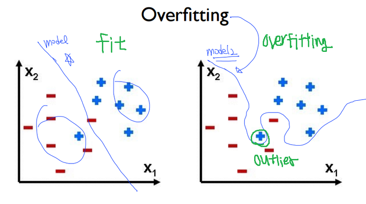
 우선 Overfitting이라는 문제점이 왜 일어나는지 그 원인에 대해서 알아보겠습니다. 오버핏팅은 위와 같이 '한정적인 데이타 셋'을 가지고 학습을 할 경우, 이러한 특정한 자료들에 특화된 W(가중치)가 도출 되면서 발생합니다. 즉, Outlier(노이즈)까지 모두 고려함으로써 오차는 줄어들겠지만, 너무 현재의 한정적인 데이터에 최적화 되어있기에 오히려 새로운 추가적인 데이터가 유입될 경우, 오차는 커지게 됩니다. 다시말해서, 학습 시 에러 값은 낮겠지만, 실제 검증 시에는 높은 에러 값을 가지게 되어서 문제가 되는 것 입니다. 

 반면에 fitting은 약간의 오차는 있지만 적절하게 Outlier를 배제함으로써 더욱 정확한 학습을 할 수 있게 됩니다. 이렇게 되면 학습과 검증시를 고려할 때, 비슷한 에러 값을 가지고 또한 그 값이 작기에, 궁극적으로 우리의 지향점이 되기도 합니다.  즉, 가장 바람직한 것은 노멀피팅이고, 현재 오버핏팅이라면 그 해결책은 규제화(Regularization) 입니다. 해결책이라고 했으니 당연히 문제의 원인이었던 아웃라이어의 영향을 최소화해주겠죠? 이제 규제화에 대해 공부해보도록 하겠습니다.

 Regularization(규제화)

1.  Affine transformation, Elastic distortion

 <첫번째> 해결방법은 '한정적인 데이터'를 늘려주는 것 입니다. 그러면 학습시에 방대한 양의 데이터 셋으로 인해서 애초에 오버핏팅의 문제는 해결될 수 도 있습니다.  한 예로 한 가지 데이터를 아래와 같이 단순 변형, 크기 조절, 휘어짐 조절을 함으로써 수 많은 데이터를 만들어낼 수 있습니다. 이를 Affine transformation 이라고 합니다.

 그 외에도 Elastic distortion는 단순 변형을 넘어 다양한 방향으로 변형을 시도하기 위해 displacement vector를 활용하기도 합니다. 하지만 데이터 셋을 늘리는 방법은 효율성 그리고 투입되는 시간 비용들을 적절히 따져봐야한다는 것 잊지 마세요!

 2. L1, L2 Regularization

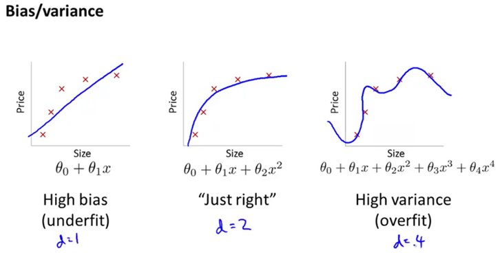
 <두번째> 방법으로는 바로 아래와 같이 노이즈들을 포함하기 위해 굴곡 졌던 로지스틱 회귀식을 곱게 펴주면서 해결이 됩니다. 위와 같이 굴곡이 많이 졌음은 곧, 로지스틱 회귀분석식이 고계 차수로 이루어졌음을 알 수 있습니다. 이러한 고계 차수들의 계수인 Weight(혹은 세타)들이 작아져야지 회귀분석식이 부드럽게 펴지는 것입니다. 다시말해서, Cost(오차)도 최소화하고 동시에 W도 작게 해줌으로써 이 문제를 해결 하는 것 입니다.

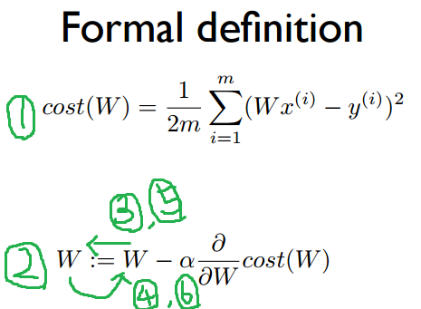
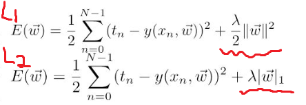
 기억을 더듬어서 Cost를 최소화하는 방법에는 무었이있었죠? 네, GradientDescent 알고리즘이 있었죠 경사감소법이라고도 합니다. 그 알고리즘을 간단하게 표현하면 위의 자료에서 2번식에 해당됩니다. 그렇다면 여기에 추가적으로 W를 작게 만들기 위해 Cost 부분에 수식을 추가할 것입니다. 그래야 2번식에서 Cost의 편미분 값이 W에 영향을 주어 작게 만들 수 있겠죠.

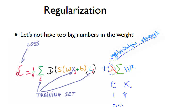
 여기서 L은 loss로써 Cost와 같습니다. 그리고 기존의 로지스틱 Cost함수에 한 개의 term이 추가 된 것 보이실 겁니다. 여기서 람다는 regularization strength로 규제화의 세기를 결정합니다. 그 값이 클 수록 규제화 강해집니다.

실제로 그 부분을 W로 편미분하여 위의 W식(2번식)에 대입을 해보면 W의 계수가  가 됩니다. 

즉, W에   가 곱해짐으로써 W는 작아지고 결국, 우리의 목적이 달성이 되는 겁니다. Weight decay라고도 합니다. 이러한 방식을 L2(Ridge regularization)이라고 합니다. 그 외에도 L1(Lasso regularization)이 있습니다. 이 둘의 차이점에 대해서 알아보겠습니다.

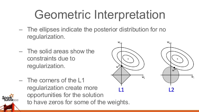
 우선 위의 자료에서 x축과 y축은 W1, W2입니다. 이해를 돕기위해서 가중치가 2가지 일 때로 생각하겠습니다. 그렇게 되면 z축은 Cost로 2차원 평면에 그린다면 위의 자료와 같이 등고선의 형태로 Cost는 나타내어 집니다. 그리고 L1과 L2에서의 마름모꼴과 원의 형태는  아래 자료의 각각 더해진 term을 보면 쉽게 이해할 수 있습니다. L1의 경우 (W1+W2)^2는 원의 형태 이고, 절댓값 W1+W2는 그래프로 그렸을 때, 마름모의 모양인 것은 당연합니다.

 즉 이러한 W1, W2가 Constraint의 역할을 하는 것입니다. 이러한 제한 조건이 있을 때, Cost는 최소가 되어야합니다. 즉 미분적분학의 Lagrange equation과 일맥상통합니다. 이를 기하학적으로 이해한다면 위의 그림자료처럼 Cost 그래프와 각각의 마름모, 원이 접할 때, Cost도 최소가 되고, W도 최소가 되는 즉, 우리가 원하는 Regularization 의 상태가 됩니다. 

 L1의 경우, 그 접하는 지점이 한 쪽 구석일 가능성이 높은데, 이것이 뜻하는 바는 W1 또는 W2 한 쪽의 가중치가 0가 된다는 뜻이고, 이처럼 영향도가 작은 노이즈 또는 아웃라이어에 대한 특성을 Regularization 과정에서 아예 배제함으로써 좀 더 중요한 특성을 강조 할 수 있게 됩니다. 반면에 L2의 경우 어느 한 쪽을 배제하지는 않고 적절하게 W1과 W2을 모두 고려하여 전체적인 Cost가 작게 만들 수 있다는 장점이 있습니다.

 3. Dropout(드롭아웃)

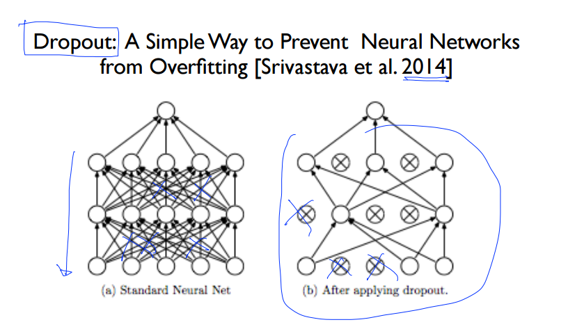
 <세번째> 방법으로는 Dropout 이 있습니다. 우선 이해를 위해서 이를 잘 정리해놓은 자료를 보겠습니다.

 Dropout은 복잡한 Neural Network에서 몇몇 Node들의 관계를 끊어버리는 것 입니다. 그럼으로써 오히려 전체적으로 보았을 때, 올바르게 학습할 수 있는다는 원리입니다. 좀 더 그 과정을 상세히 설명한다면, input layer와 hidden layer에 있는 node를 dropout_rate 만큼 제거를 해버립니다. 제거의 기준은 랜덤형식입니다. 그런 상태에서 학습을 끝내고, 본래 dropout은 Regularization의 용도였으니, 검증시에는 본래의 노드를 모두 사용합니다. 대신에 검증(test)시에는 노드가 제거되지 않았던 원상태의 노드의 Weight에 dropout_rate를 곱해서 학습한 결과를 반영하는 방식입니다.

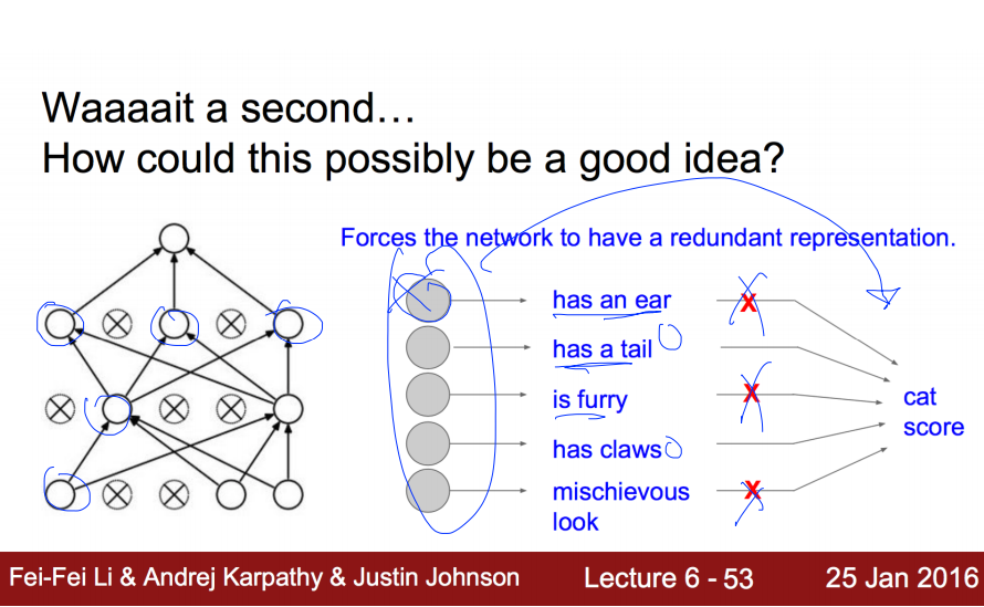
 예를 들어서, 고양이를 인식할 때, 각각의 노드들을 전문가라고 생각해봅시다. 각각의 전문가들의 묘사를 듣고서는 오히려 설명하는 객체가 무었인지 혼란스러울 수 있습니다. 이 것이 바로 Overfitting 입니다. 그 해결책으로 몇몇의 전문가들의 의견을 1차적으로 수렴하고 다음번에는 다른 몇몇의 전문가들의 의견을 수렴하는 방법; 그래서 설명하는 객체가 고양이임을 더 정확하게 파악할 수 있다.  바로 이것이 dropout 입니다. 파이썬으로 구현시 dropout_rate = 0.7 이라면 30%의 노드간의 연결은 끊겟다고 해석하시면 됩니다.

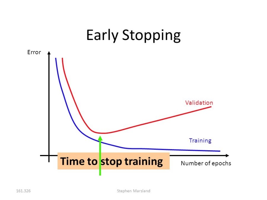
 4. Early stopping(얼리스탑핑)

 <네번째> 방법으로는 Early stopping(얼리스탑핑)이 있습니다. 이 방법은 현재의 '한정적인 테이터 셋'을 Training set, Validation set, Test set 이렇게 3개 영역으로 나누어서 먼저 Training set으로만 학습을 시킵니다. 그런 후, Validation set을 새로운 데이터인 것 처럼 조금씩 추가적으로 학습을 시킵니다. 그러다 보면 어느 순간, 이미 Training set에 최적화된 로지스틱 함수이기에, 에러가 어느 순간 부터 증가하기 시작할 겁니다. 즉, Overfitting 현상이 일어납니다. 그러면 우리는 그 순간에 학습을 stop 시키는 것 입니다. 그런 후, 마지막으로 우리는 Test set으로 남겨두었던 데이터로 final evaluation(검증)을 실시합니다. 그림으로 이해해보겠습니다.

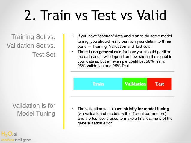
 이 방법의 특징은 '한정적인 데이터 셋'을 세가지의 영역으로 나누어서, 마치 Validation과 Test 데이터는 남겨두어 현실에서 얻은 새로운 데이터인 것처럼 취급합니다. 세 영역으로 나누는 ratio에 있어서  general rule은 없으나 보통 Train(50%), Validation(25%), Test(25%)의 비율로 나눕니다. 60%, 20%, 20% 도 많이 쓰이며 data가 별로 없을 때는(ex 300 data) test data set은 배제하고 2/3를 Train에 그리고 1/3을 Validation에 배정하기도 합니다. 

  이 방법의 실효성을 위해서는 Test set은 현실의 데이터를 잘 대표 할 수 있어야하고, Validation set 또한 Test set을 잘 대표 할 수 있어야합니다. 쉽게 정리하자면, Train data set으로 먼저 학습을 시킨 후, 로지스틱 회귀식을 얻어냅니다. 그런 후, tuning의 목적으로 남겨둔 validation data set으로 early stopping을 적용합니다. 그런 후, 마지막 evaluation으로써 Test data set으로 검증을 실시 합니다. 

<Summary>

 이렇게 오늘은 Overfitting의 원인과 해결방법에 대해서 공부해보았습니다. 그 원인은 '한정된 데이터 셋'으로 Cost를 최소화하는데 집중하다보니 아웃라이어에 민감하게 되었고 특정 Weight들이 커지게 되어서, 로지스틱 회귀식이 굴곡지게 되는 것입니다. 그러다 보니 현재의 데이터에는 완벽하게 Cost가 작아지게 W가 학습되었지만, 실제 추가적인 데이터로 검증시에는 Cost가 급증하게 되었습니다

이러한 오버피팅을 해결하는 방법에는 

1. 양질의 데이터를 늘리는 것 - 시간, 비용을 따져봐야합니다. 

2. Regularization의 방법을 통해 Cost를 줄임과 동시에 Weight도 줄이는 해결책이 있습니다. 대표적인 방법으로 L1, L2 가 있습니다.

3. Dropout 적절하게 각 노드간의 연결을 끊음으로써 더욱 정확하게 학습 할 수 있다는 원리이었습니다.

4. Early stopping - Validation set 으로 학습하면서 error가 급증하는 순간 학습을 멈춥니다.

Reference

http://www.coursera.org/learn/machine-learning/

http://hunkim.github.io/ml/lec7.pdf

http://slideplayer.com/slide/3415513/

http://www.slideshare.net/0xdata/top-10-data-science-practitioner-pitfalls

http://slideplayer.com/slide/5008746/

http://www.slideshare.net/dbtsai/2015-06-largescale-lasso-and-elasticnet-regularized-generalized-linear-models-at-spark-summit

https://www.quora.com/What-are-C-and-gamma-with-regards-to-a-support-vector-machine

C: regularization parameter. 즉, C가 크면 아주 strict하게 나누고, 작으면, 오판된 데이터를 잘 허용한다

gamma: window size for gaussian kernel. r = 1/(2*sigma^2). 따라서, sigma가 크면(gamma가 작으면) 윈도우 사이즈가 커져서 support vector의 영향력이 크게 된다.

Jeffrey M GirardPsychology PhD Student

Studied at University of Pittsburgh

Lives in Pittsburgh, PA

291.5k answer views12k this month

Most Viewed Writer

Facial Expressions,

Support Vector Machines

Jeffrey M Girard, Affective Computing Researcher

Updated Apr 23, 2016

C and Gamma are the parameters for a nonlinear support vector machine (SVM) with a Gaussian radial basis function kernel.

A standard SVM seeks to find a margin that separates all positive and negative examples. However, this can lead to poorly fit models if any examples are mislabeled or extremely unusual. To account for this, in 1995, Cortes and Vapnik proposed the idea of a "soft margin" SVM that allows some examples to be "ignored" or placed on the wrong side of the margin; this innovation often leads to a better overall fit. C is the parameter for the soft margin cost function, which controls the influence of each individual support vector; this process involves trading error penalty for stability.

From: SVM - hard or soft margins?

A standard SVM is a type of linear classification using dot product. However, in 1992, Boser, Guyan, and Vapnik proposed a way to model more complicated relationships by replacing each dot product with a nonlinear kernel function (such as a Gaussian radial basis function or Polynomial kernel). Gamma is the free parameter of the Gaussian radial basis function.

A small gamma means a Gaussian with a large variance so the influence of x_j is more, i.e. if x_j is a support vector, a small gamma implies the class of this support vector will have influence on deciding the class of the vector x_i even if the distance between them is large. If gamma is large, then variance is small implying the support vector does not have wide-spread influence. Technically speaking, large gamma leads to high bias and low variance models, and vice-versa.

http://stackoverflow.com/questions/22916915/parameter-settings-for-neural-networks-based-classification-using-matlab

Parameter settings for neural networks based classification using Matlab

Recently, I am trying to using Matlab build-in neural networks toolbox to accomplish my classification problem. However, I have some questions about the parameter settings.

a. The number of neurons in the hidden layer:

The example on this page Matlab neural networks classification example shows a two-layer (i.e. one-hidden-layer and one-output-layer) feed forward neural networks. In this example, it uses 10 neurons in the hidden layer

net = patternnet(10);

My first question is how to define the best number of neurons for my classification problem? Should I use cross-validation method to get the best performed number of neurons using a training data set?

b. Is there a method to choose three-layer or more multi-layer neural networks?

c. There are many different training method we can use in the neural networks toolbox. A list can be found at Training methods list. The page mentioned that the fastest training function is generally 'trainlm'; however, generally speaking, which one will perform best? Or it totally depends on the data set I am using?

d. In each training method, there is a parameter called 'epochs', which is the training iteration for my understanding. For each training method, Matlab defined the maximum number of epochs to train. However, from the example, it seems like 'epochs' is another parameter we can tune. Am I right? Or we just set the maximum number of epochs or leave it as default?

Any experience with Matlab neural networks toolbox is welcome and thanks very much for your reply. A.

------------------------------------------------------------------

a. You can refer to How to choose number of hidden layers and nodes in neural network? and ftp://ftp.sas.com/pub/neural/FAQ3.html#A_hu
Surely you can do cross-validation to determine the parameter of best number of neurons. But it's not recommended as it's more suitable to use it in the stage of weights training of a certain network.

b. Refer to ftp://ftp.sas.com/pub/neural/FAQ3.html#A_hl
And for more layers of neural network, you can refer to Deep Learning, which is very hot in recent years and gets state-of-the-art performances in many of the pattern recognition tasks.

c. It depends on your data. trainlm performs better on function fitting (nonlinear regression) problems than on pattern recognition problems while training large networks and pattern recognition networks, trainscg and trainrp are good choices. Generally, Gradient Descent and Resilient Backpropagation is recommended. More detailed comparison can be found here: http://www.mathworks.cn/cn/help/nnet/ug/choose-a-multilayer-neural-network-training-function.html

d. Yes, you're right. We can tune the epochs parameter. Generally you can output the recognition results/accuracy at every epoch and you will see that it is promoting more and more slowly, and the more epochs the more computing time. You can make a compromise between the accuracy and computation time.

For part b of your question: You can use like this code:

net = patternnet([10 15 20]);

This script create a network with 3 hidden layer that first layer has 10 neurons, second layer has 15 neurons and 3th layer has 20 neurons.

Domain-Adaptation.pdf