matlab code - convert face landmarks matlab .mat to .pts file
excute 'main_trans_mat2pts_20180607_openVer.m' in matlab
 trans_mat2pts_openVer.zip
matlab code - convert face landmarks matlab .mat to .pts file
excute 'main_trans_mat2pts_20180607_openVer.m' in matlab
https://www.mathworks.com/matlabcentral/answers/341643-how-to-convert-a-mp3-to-wav-file-in-matlab
https://www.mathworks.com/matlabcentral/answers/160834-extracting-a-segment-from-sound-file
https://www.mathworks.com/matlabcentral/answers/323480-how-to-cut-audio-file-into-segments
https://stackoverflow.com/questions/37352712/read-wav-segment-in-matlab
https://stackoverflow.com/questions/29905701/splitting-an-audio-file-in-matlab
https://kr.mathworks.com/help/images/ref/imhistmatch.html
imhistmatch
Adjust histogram of 2-D image to match histogram of reference image
B = imhistmatch(A,ref)B = imhistmatch(A,ref,nbins)[B,hgram] = imhistmatch(___)B = imhistmatch(A,ref)A returning output image B whose histogram approximately matches the histogram of the reference image ref.
If both A and ref are truecolor RGB images, imhistmatch matches each color channel of A independently to the corresponding color channel of ref.
If A is a truecolor RGB image and ref is a grayscale image, imhistmatch matches each channel of A against the single histogram derived from ref.
If A is a grayscale image, ref must also be a grayscale image.
Images A and ref can be any of the permissible data types and need not be equal in size.
B = imhistmatch(A,ref,nbins)nbins equally spaced bins within the appropriate range for the given image data type. The returned image B has no more than nbins discrete levels.
If the data type of the image is either single or double, the histogram range is [0, 1].
If the data type of the image is uint8, the histogram range is [0, 255].
If the data type of the image is uint16, the histogram range is [0, 65535].
If the data type of the image is int16, the histogram range is [-32768, 32767].
[ returns the histogram of the reference image B,hgram] = imhistmatch(___)ref used for matching in hgram. hgram is a 1-by-nbins (when ref is grayscale) or a 3-by-nbins (when ref is truecolor) matrix, where nbins is the number of histogram bins. Each row in hgram stores the histogram of a single color channel of ref.
These aerial images, taken at different times, represent overlapping views of the same terrain in Concord, Massachusetts. This example demonstrates that input images A and Ref can be of different sizes and image types.
Load an RGB image and a reference grayscale image.
A = imread('concordaerial.png');
Ref = imread('concordorthophoto.png');
Get the size of A.
size(A)
ans =

        2036        3060           3
Get the size of Ref.
size(Ref)
ans =

        2215        2956
Note that image A and Ref are different in size and type. Image A is a truecolor RGB image, while image Ref is a grayscale image. Both images are of data type uint8.
Generate the histogram matched output image. The example matches each channel of A against the single histogram of Ref. Output image B takes on the characteristics of image A - it is an RGB image whose size and data type is the same as image A. The number of distinct levels present in each RGB channel of image B is the same as the number of bins in the histogram built from grayscale image Ref. In this example, the histogram of Ref and B have the default number of bins, 64.
B = imhistmatch(A,Ref);
Display the RGB image A, the reference image Ref, and the histogram matched RGB image B. The images are resized before display.
figure
imshow(imresize(A, 0.25))
title('RGB Image with Color Cast')
figure
imshow(imresize(Ref, 0.25))
title('Reference Grayscale Image')
figure
imshow(imresize(B, 0.25))
title('Histogram Matched RGB Image')
In this example, you will see the effect on output image B of varying the number of equally spaced bins in the target histogram of image Ref, from its default value 64 to the maximum value of 256 for uint8 pixel data.
The following images were taken with a digital camera and represent two different exposures of the same scene.
    A   = imread('office_2.jpg');   % Dark Image
    Ref = imread('office_4.jpg');   % Reference image
Image A, being the darker image, has a preponderance of its pixels in the lower bins. The reference image, Ref, is a properly exposed image and fully populates all of the available bins values in all three RGB channels: as shown in the table below, all three channels have 256 unique levels for 8–bit pixel values.

The unique 8-bit level values for the red channel is 205 for A and 256 for Ref. The unique 8-bit level values for the green channel is 193 for A and 256 for Ref. The unique 8-bit level values for the blue channel is 224 for A and 256 for Ref.
The example generates the output image B using three different values of nbins: 64, 128 and 256. The objective of function imhistmatch is to transform image A such that the histogram of output image B is a match to the histogram of Ref built with nbins equally spaced bins. As a result, nbins represents the upper limit of the number of discrete data levels present in image B.
[B64,  hgram] = imhistmatch(A, Ref,  64);
[B128, hgram] = imhistmatch(A, Ref, 128);
[B256, hgram] = imhistmatch(A, Ref, 256);

The unique 8-bit level values for the red channel for nbins=[64 128 256] are 57 for output image B64, 101 for output image B128, and 134 for output image B256. The unique 8-bit level values for the green channel for nbins=[64 128 256] are 57 for output image B64, 101 for output image B128, and 134 for output image B256. The unique 8-bit level values for the blue channel for nbins=[64 128 256] are 57 for output image B64, 101 for output image B128, and 134 for output image B256. Note that as nbins increases, the number of levels in each RGB channel of output image B also increases.
This example shows how to perform histogram matching with different numbers of bins.
Load a 16-bit DICOM image of a knee imaged via MRI.
K = dicomread('knee1.dcm');   % read in original 16-bit image
LevelsK = unique(K(:));       % determine number of unique code values
disp(['image K: ',num2str(length(LevelsK)),' distinct levels']);
image K: 448 distinct levels
disp(['max level = ' num2str( max(LevelsK) )]);max level = 473
disp(['min level = ' num2str( min(LevelsK) )]);min level = 0
All 448 discrete values are at low code values, which causes the image to look dark. To rectify this, scale the image data to span the entire 16-bit range of [0, 65535].
Kdouble = double(K);                  % cast uint16 to double
kmult = 65535/(max(max(Kdouble(:)))); % full range multiplier
Ref = uint16(kmult*Kdouble);   % full range 16-bit reference image
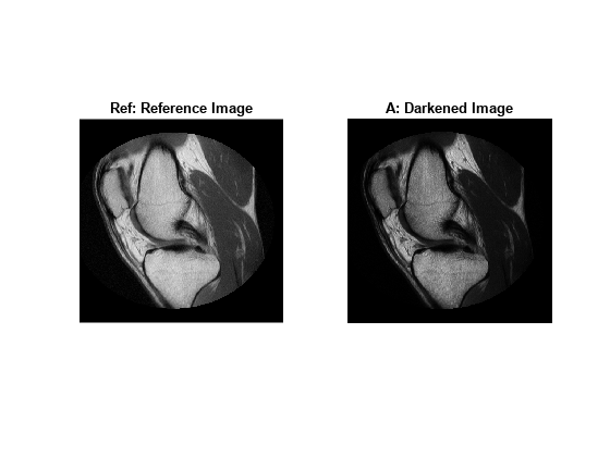
Darken the reference image Ref to create an image A that can be used in the histogram matching operation.
%Build concave bow-shaped curve for darkening |Ref|.
ramp = [0:65535]/65535;
ppconcave = spline([0 .1 .50  .72 .87 1],[0 .025 .25 .5 .75 1]);
Ybuf = ppval( ppconcave, ramp);
Lut16bit = uint16( round( 65535*Ybuf ) );
% Pass image |Ref| through a lookup table (LUT) to darken the image.
A = intlut(Ref,Lut16bit);
View the reference image Ref and the darkened image A. Note that they have the same number of discrete code values, but differ in overall brightness.
subplot(1,2,1)
imshow(Ref)
title('Ref: Reference Image')
subplot(1,2,2)
imshow(A)
title('A: Darkened Image');
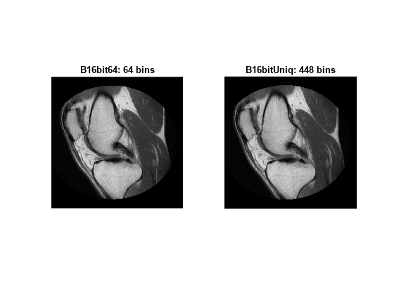
Generate histogram-matched output images using histograms with different number of bins. First use the default number of bins, 64. Then use the number of values present in image A, 448 bins.
B16bit64 = imhistmatch(A(:,:,1),Ref(:,:,1));  % default: 64 bins

N = length(LevelsK);     % number of unique 16-bit code values in image A.
B16bitUniq = imhistmatch(A(:,:,1),Ref(:,:,1),N);
View the results of the two histogram matching operations.
figure
subplot(1,2,1)
imshow(B16bit64)
title('B16bit64: 64 bins')
subplot(1,2,2)
imshow(Ref)
title(['B16bitUniq: ',num2str(N),' bins'])
The objective of imhistmatch is to transform image A such that the histogram of image B matches the histogram derived from image ref. It consists of nbins equally spaced bins which span the full range of the image data type. A consequence of matching histograms in this way is that nbins also represents the upper limit of the number of discrete data levels present in image B.
An important behavioral aspect of this algorithm to note is that as nbins increases in value, the degree of rapid fluctuations between adjacent populated peaks in the histogram of image B tends to increase. This can be seen in the following histogram plots taken from the 16–bit grayscale MRI example.

An optimal value for nbins represents a trade-off between more output levels (larger values of nbins) while minimizing peak fluctuations in the histogram (smaller values of nbins).
histeq | imadjust | imhist | imhistmatchn
| matlab code - convert face landmarks matlab .mat to .pts file (0) | 2018.06.07 |
|---|---|
| matlab audio read write (0) | 2017.12.20 |
| matlab figure 파일을 300dpi로 저장하는 법 - How can I save a figure to a TIFF image with resolution 300 dpi in MATLAB? (0) | 2017.03.27 |
| matlab TreeBagger 예제 나와있는 페이지 (0) | 2017.03.11 |
| MATLAB Treebagger and Random Forests (0) | 2017.03.11 |
1. https://www.mathworks.com/matlabcentral/fileexchange/6626-passive-mode-ftp-in-matlab?focused=5174243&tab=function에서 프로그램을 다운받는다
2. matlab prompt에 'which ftp'라고 입력하여 built-in ftp함수가 있는 폴더를 알아낸다.
나의 경우엔,
C:\Program Files\MATLAB\R2016a\toolbox\matlab\iofun\@ftp\ftp.m % ftp constructor
3. C:\Program Files\MATLAB\R2016a\toolbox\matlab\iofun 로 이동하여 @ftp라는 폴더를 복사하여 임의의 폴더에 저장한다. e.g., C:\myWork\myFunctions\@ftp
4. matlab prompt에 아래와 같이 입력하여 path를 저장한다
addpath('C:\myWork\myFunctions')
savepath
5. PassiveFTP/connect.m 을 'C:\myWork\myFunctions/@ftp/private/'에 복사한다
6. PassiveFTP/active.m dataMode.m ftp.m pasv.m 을 'C:\myWork\myFunctions/@ftp/에 복사한다.
7. matlab을 종료했다가 다시 실행한 후, rehash toolboxcache을 입력한다.
8.
myFTP = ftp('ftp.mathworks.com')
pasv(myFTP)
dataMode(myFTP) % this command simply shows the current mode
you can return to normal/active mode by issuing the command
active(myFTP)
| This collection of over 300 MATLAB examples can help you with image processing and computer vision problems (0) | 2017.03.31 |
|---|---|
| Top 10 most popular MATLAB & Simulink file downloads from last year (0) | 2017.03.18 |
| random forest using matlab (0) | 2017.03.12 |
| Some Matlab Code (0) | 2017.03.07 |
| plot standard deviation and mean (0) | 2017.02.08 |
| Passive Mode FTP in MATLAB (0) | 2017.04.04 |
|---|---|
| Top 10 most popular MATLAB & Simulink file downloads from last year (0) | 2017.03.18 |
| random forest using matlab (0) | 2017.03.12 |
| Some Matlab Code (0) | 2017.03.07 |
| plot standard deviation and mean (0) | 2017.02.08 |
matlab figure 파일을 300dpi로 저장하는 법
1. Using the MATLAB Graphical Environment
Select the figure window that shows the figure to be saved and then follow the steps mentioned below:
- ‘Colorspace’ to ’grayscale’
- ‘Resolution(dpi)’ to 300
This step is shown in image file “Step3.jpeg” attached to the solution.
2. Saving a figure to an image file programmatically
a) Use "print" as:
>> print(gcf, '-dtiff', 'myfigure.tiff');
b) Alternatively, you could do:
>> imagewd = getframe(gcf);
>> imwrite(imagewd.cdata, 'myfigure.tiff');
To change the quality of a TIFF file, you can specify 'Compression',''none' and increase the resolution with 'Resolution',300.
| matlab audio read write (0) | 2017.12.20 |
|---|---|
| imhistmatch - Adjust histogram of 2-D image to match histogram of reference image 테스트 영상 히스토그램을 reference영상 히스토그램으로 바꿔주는 함수 (0) | 2017.07.04 |
| matlab TreeBagger 예제 나와있는 페이지 (0) | 2017.03.11 |
| MATLAB Treebagger and Random Forests (0) | 2017.03.11 |
| Tune Random Forest Using Quantile Error and Bayesian Optimization (0) | 2017.03.11 |
| Passive Mode FTP in MATLAB (0) | 2017.04.04 |
|---|---|
| This collection of over 300 MATLAB examples can help you with image processing and computer vision problems (0) | 2017.03.31 |
| random forest using matlab (0) | 2017.03.12 |
| Some Matlab Code (0) | 2017.03.07 |
| plot standard deviation and mean (0) | 2017.02.08 |
| This collection of over 300 MATLAB examples can help you with image processing and computer vision problems (0) | 2017.03.31 |
|---|---|
| Top 10 most popular MATLAB & Simulink file downloads from last year (0) | 2017.03.18 |
| Some Matlab Code (0) | 2017.03.07 |
| plot standard deviation and mean (0) | 2017.02.08 |
| matlab dist function (0) | 2017.01.17 |
https://github.com/mlab-upenn/DRAdvisor
https://github.com/mlab-upenn/DRAdvisor/blob/master/Tool/GUI/Inputs.m
| B = TreeBagger(num_trees,Xtrain,Ytrain,'Method','regression','OOBPred','On','OOBVarImp','on',... | |
| 'CategoricalPredictors',catcol,'MinLeaf',minleaf); |
http://stackoverflow.com/questions/17549337/matlab-treebagger-and-random-forests
Does the Treebagger class in MATLAB apply Breiman's Random Forest algorithm?
If I simply use Treebagger, is it the same as using Random Forests, or do I need to modify some parameters?
Thanks.
TreeBagger implements a bagged decision tree algorithm, rather than Random Forests specifically.
You can get TreeBagger to behave basically the same as Random Forests as long as the NVarsToSample parameter is set appropriately. See the documentation page for TreeBagger, under the NVarsToSample parameter, for details.
Edit: Note that in release R2015b, the NVarsToSample parameter has been renamed to NumPredictorsToSample.
http://stats.stackexchange.com/questions/184589/random-forests-for-predictor-importance-matlab
What you describe would be one approach. For classification, TreeBagger by default randomly selects sqrt(p) predictors for each decision split (setting recommended by Breiman).
| matlab figure 파일을 300dpi로 저장하는 법 - How can I save a figure to a TIFF image with resolution 300 dpi in MATLAB? (0) | 2017.03.27 |
|---|---|
| matlab TreeBagger 예제 나와있는 페이지 (0) | 2017.03.11 |
| Tune Random Forest Using Quantile Error and Bayesian Optimization (0) | 2017.03.11 |
| matlab fitcnb( naive Bayes model) parameter tuning방법 (0) | 2017.03.11 |
| matlab fitglm function parameter tuning references (0) | 2017.03.09 |
This example shows how to implement Bayesian optimization to tune the hyperparameters of a random forest of regression trees using quantile error. Tuning a model using quantile error, rather than mean squared error, is appropriate if you plan to use the model to predict conditional quantiles rather than conditional means.
Load the carsmall data set. Consider a model that predicts the median fuel economy of a car given its acceleration, number of cylinders, engine displacement, horsepower, manufacturer, model year, and weight. Consider Cylinders, Mfg, and Model_Year as categorical variables.
load carsmall
Cylinders = categorical(Cylinders);
Mfg = categorical(cellstr(Mfg));
Model_Year = categorical(Model_Year);
X = table(Acceleration,Cylinders,Displacement,Horsepower,Mfg,...
    Model_Year,Weight,MPG);
rng('default'); % For reproducibility
Consider tuning:
The complexity (depth) of the trees in the forest. Deep trees tend to over-fit, but shallow trees tend to underfit. Therefore, specify that the minimum number of observations per leaf be at most 20.
When growing the trees, the number of predictors to sample at each node. Specify sampling from 1 through all of the predictors.
bayesopt, the function that implements Bayesian optimization, requires you to pass these specifications as optimizableVariable objects.
maxMinLS = 20;
minLS = optimizableVariable('minLS',[1,maxMinLS],'Type','integer');
numPTS = optimizableVariable('numPTS',[1,size(X,2)-1],'Type','integer');
hyperparametersRF = [minLS; numPTS];
hyperparametersRF is a 2-by-1 array of OptimizableVariable objects.
You should also consider tuning the number of trees in the ensemble. bayesopt tends to choose random forests containing many trees because ensembles with more learners are more accurate. If available computation resources is a consideration, and you prefer ensembles with as fewer trees, then consider tuning the number of trees separately from the other parameters or penalizing models containing many learners.
Declare an objective function for the Bayesian optimization algorithm to optimize. The function should:
Accept the parameters to tune as an input.
Train a random forest using TreeBagger. In the TreeBagger call, specify the parameters to tune and specify returning the out-of-bag indices.
Estimate the out-of-bag quantile error based on the median.
Return the out-of-bag quantile error.
function oobErr = oobErrRF(params,X)
%oobErrRF Trains random forest and estimates out-of-bag quantile error
%   oobErr trains a random forest of 300 regression trees using the
%   predictor data in X and the parameter specification in params, and then
%   returns the out-of-bag quantile error based on the median. X is a table
%   and params is an array of OptimizableVariable objects corresponding to
%   the minimum leaf size and number of predictors to sample at each node.
randomForest = TreeBagger(300,X,'MPG','Method','regression',...
    'OOBPrediction','on','MinLeafSize',params.minLS,...
    'NumPredictorstoSample',params.numPTS);
oobErr = oobQuantileError(randomForest);
end
Find the model achieving the minimal, penalized, out-of-bag quantile error with respect to tree complexity and number of predictors to sample at each node using Bayesian optimization. Specify the expected improvement plus function as the acquisition function and suppress printing the optimization information.
results = bayesopt(@(params)oobErrRF(params,X),hyperparametersRF,...
    'AcquisitionFunctionName','expected-improvement-plus','Verbose',0);
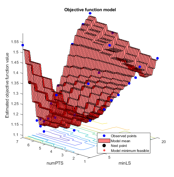
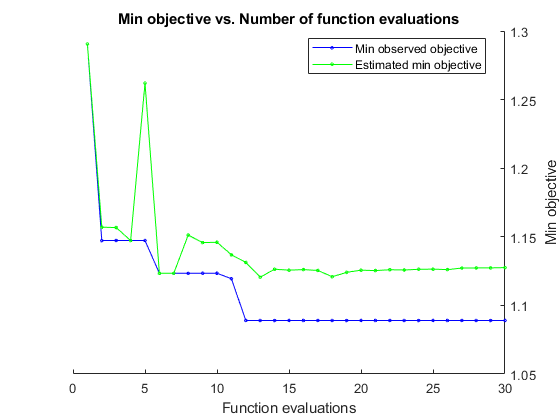
results is a BayesianOptimization object containing, among other things, the minimum of the objective function and the optimized hyperparameter values.
Display the observed minimum of the objective function and the optimized hyperparameter values.
bestOOBErr = results.MinObjective
bestHyperparameters = results.XAtMinObjective
bestOOBErr =

    1.1207


bestHyperparameters =

  1×2 table

    minLS    numPTS
    _____    ______

    7        6
Train a random forest using the entire data set and the optimized hyperparameter values.
Mdl = TreeBagger(300,X,'MPG','Method','regression',...
    'MinLeafSize',bestHyperparameters.minLS,...
    'NumPredictorstoSample',bestHyperparameters.numPTS);
Mdl is TreeBagger object optimized for median prediction. You can predict the median fuel economy given predictor data by passing Mdl and the new data to quantilePredict.
| matlab TreeBagger 예제 나와있는 페이지 (0) | 2017.03.11 |
|---|---|
| MATLAB Treebagger and Random Forests (0) | 2017.03.11 |
| matlab fitcnb( naive Bayes model) parameter tuning방법 (0) | 2017.03.11 |
| matlab fitglm function parameter tuning references (0) | 2017.03.09 |
| Difference between 'link function' and 'canonical link function' for GLM (0) | 2017.03.08 |
'DistributionNames' = {'kernel', 'mn', 'mvmn', 'normal'}; %
'DistributionNames'을 'kernel'을 선택할 경우, {'normal', 'box', 'epanechnikov', 'triangle'}중에서 하나 골라야하고, 나머지 'mn', 'mvmn', 'normal'중 하나일경우에는 'Kernel'은 설정하지 않는다.
| MATLAB Treebagger and Random Forests (0) | 2017.03.11 |
|---|---|
| Tune Random Forest Using Quantile Error and Bayesian Optimization (0) | 2017.03.11 |
| matlab fitglm function parameter tuning references (0) | 2017.03.09 |
| Difference between 'link function' and 'canonical link function' for GLM (0) | 2017.03.08 |
| matlab feval VS predict (0) | 2017.03.07 |
http://d-scholarship.pitt.edu/8524/1/01ZhaoMYdissertation.pdf
https://esc.fnwi.uva.nl/thesis/centraal/files/f993098462.pdf
Numerical methods using matlab
| Tune Random Forest Using Quantile Error and Bayesian Optimization (0) | 2017.03.11 |
|---|---|
| matlab fitcnb( naive Bayes model) parameter tuning방법 (0) | 2017.03.11 |
| Difference between 'link function' and 'canonical link function' for GLM (0) | 2017.03.08 |
| matlab feval VS predict (0) | 2017.03.07 |
| MATLAB's glmfit vs fitglm , difference (0) | 2017.03.07 |
| matlab fitcnb( naive Bayes model) parameter tuning방법 (0) | 2017.03.11 |
|---|---|
| matlab fitglm function parameter tuning references (0) | 2017.03.09 |
| matlab feval VS predict (0) | 2017.03.07 |
| MATLAB's glmfit vs fitglm , difference (0) | 2017.03.07 |
| Is there any function to calculate Precision and Recall using Matlab? (0) | 2017.03.07 |
feval allows you to easily evaluate predictions of a model when the model was fitted using a table or dataset array. predict requires a table or dataset array with the same predictor names, but you can use simple arrays of scalars with feval.
| matlab fitglm function parameter tuning references (0) | 2017.03.09 |
|---|---|
| Difference between 'link function' and 'canonical link function' for GLM (0) | 2017.03.08 |
| MATLAB's glmfit vs fitglm , difference (0) | 2017.03.07 |
| Is there any function to calculate Precision and Recall using Matlab? (0) | 2017.03.07 |
| matlab에서 SVM으로 ROC curve 그릴 때 필요한 score(posterior probability)를 구하는 방법 (0) | 2017.03.04 |
I'm trying to perform logistic regression to do classification using MATLAB. There seem to be two different methods in MATLAB's statistics toolbox to build a generalized linear model 'glmfit' and 'fitglm'. I can't figure out what the difference is between the two. Is one preferable over the other?
Here are the links for the function descriptions.
http://uk.mathworks.com/help/stats/glmfit.html http://uk.mathworks.com/help/stats/fitglm.html
|
The difference is what the functions output. |
| Difference between 'link function' and 'canonical link function' for GLM (0) | 2017.03.08 |
|---|---|
| matlab feval VS predict (0) | 2017.03.07 |
| Is there any function to calculate Precision and Recall using Matlab? (0) | 2017.03.07 |
| matlab에서 SVM으로 ROC curve 그릴 때 필요한 score(posterior probability)를 구하는 방법 (0) | 2017.03.04 |
| Why do I receive the error "License Manager Error -9"? (0) | 2017.02.23 |


|
I have problem about calculating the precision and recall for classifier in matlab. I use fisherIris data (that consists of 150 datapoints, 50-setosa, 50-versicolor, 50-virginica). I have classified using kNN algorithm. Here is my confusion matrix: correct classification rate is 96% (144/150), but how to calculate precision and recall using matlab, is there any function? I know the formulas for that precision=tp/(tp+fp),and recall=tp/(tp+fn), but I am lost in identifying components. For instance, can I say that true positive is 144 from the matrix? what about false positive and false negative? Please help!!! I would really appreciate! Thank you! | |||||||||||||||||||||
|
|
To add to pederpansen's answer, here are some anonymous Matlab functions for calculating precision, recall and F1-score for each class, and the mean F1 score over all classes: | |||||
|
|
As Dan pointed out in his comment, precision and recall are usually defined for binary classification problems only. But you can calculate precision and recall separately for each class. Let's annotate your confusion matrix a little bit: Here I assumed the usual convention holds, i.e. columns are used for true values and rows for values predicted by your learning algorithm. (If your matrix was built the other way round, simply take the transpose of the confusion matrix.) The true positives ( If we define false positives ( Here I used the class names instead of the row indices for illustration. Please have a look at the answers to this question for further information on performance measures in the case of multi-class classification problems - particularly if you want to end up with single number instead of one number for each class. Of course, the easiest way to do this is just averaging the values for each class. UpdateI realized that you were actually looking for a Matlab function to do this. I don't think there is any built-in function, and on the Matlab File Exchange I only found a function for binary classification problems. However, the task is so easy you can easily define your own functions like so: This will return a column vector containing the precision and recall values for each class, respectively. Now you can simply call to obtain the average precision and recall values of your model. |
| matlab feval VS predict (0) | 2017.03.07 |
|---|---|
| MATLAB's glmfit vs fitglm , difference (0) | 2017.03.07 |
| matlab에서 SVM으로 ROC curve 그릴 때 필요한 score(posterior probability)를 구하는 방법 (0) | 2017.03.04 |
| Why do I receive the error "License Manager Error -9"? (0) | 2017.02.23 |
| check whether have another matlab function somewhere on your path (0) | 2017.02.22 |
This collection of Matlab code is brought to you by the phrases "caveat emptor" and "quid quid latine dictum sit, altum videtur", and by the number 404.
batchtest.m : Runs batches of train+test tasks using LIBSVM (Chang & Lin 2000), including model selection for the RBF kernel. Uses svmlwrite.m (by Anton Schwaighofer) and getcm.m. If you ask for class probability estimates, you will also need readprobest.m.
nfolds.m : Combines makefolds.m and batchtest.m
readprobest.m : Reads class probability estimates output when you use the "-b" option with LIBSVM.
splitbysomething.m : Like batchtest, but allows you to create different classifiers for different partitions of all the data. It requires the function ispartition.m.
makefolds.m : creates indices of train and test sets for each of n folds for deterministic cross-validation.
makesplits.m : partitions a vector by its values. makefolds could be made shorter if it made calls to makesplits, but I'm not going to change that (now).
getcm.m : Gets confusion matrices, accuracy, precision, recall, F-score, from actual and predicted labels.
precrec.m : Produces precision-recall and ROC curves given true labels and real-valued classifier output. Only for binary classifiers. Uses getcm.
choosebestscore.m : Chooses highest score (given precomputed scores) of elements in sequences.
revhmm.m : Does Viterbi decoding given posteriors.
KADRE.zip : Kick-ass dimensionality reduction (versions of Laplacian Eigenmaps and Isomap that use the Cover Tree algorithm to create the nearest neighbor graph... covertree code only works on linux)
makepitchtier.m : creates PitchTier file (for Praat) given measurement times and values.
Ndaona : package for producing partiview files for interactive 3d or 3d+time models
partiviewangles.m Calculates coordinates Rx and Ry required by Partiview to position a camera. (Very useful.... but use tfm.pl instead.)
For a description of the SEQ (and FLAT) formats that I use to store data for sequential classification, see my Sequential Data / Classification page.
seqread.m : reads from a file with SEQ data to a SEQ Matlab structure.
seqread.m : writes to a file with SEQ data from a SEQ Matlab structure.
seq2flat : converts from a SEQ Matlab structure to a FLAT Matlab structure.
seqkeepcols.m : converts from a SEQ Matlab structure to another SEQ Matlab structure but with only selected columns.
For a description of the PWS (Phrase-Word-Syllable) format that I use to store data for tone recognition, see my Tone Recognition page.
pws2textgrid.m : creates Praat-formatted TextGrid files, with three tiers for Phrase, Word, and Syllable, of a PWS structure (or a cell array thereof).
textgrid2pws.m : reads Praat-formatted TextGrid files into a PWS structure. Good for replacing automatic alignments with manually corrected alignments. (Remember to press SHIFT while doing the manual alignment so that boundaries across different tiers remain aligned!)
| Top 10 most popular MATLAB & Simulink file downloads from last year (0) | 2017.03.18 |
|---|---|
| random forest using matlab (0) | 2017.03.12 |
| plot standard deviation and mean (0) | 2017.02.08 |
| matlab dist function (0) | 2017.01.17 |
| matlab de2bi source code (0) | 2017.01.17 |
matlab에서 fitcsvm함수로 SVM분류기를 이용해 ROC curve를 그리려면, 학습한 SVM 모델을 fitPosterior함수(score 를 posterior probability로 변환)를 통해 모델을 변환한 후 predict함수의 입력모델로 써야 해줘야 test셋의 posterior probability를 구할 수 있다. 이 posterior probability를 perfcurve에 입력시켜 roc curve와 auc를 그릴 수 있다. 아래는 그 예제.
 test_fitcsvm_predict_perfcurve1.m
close all; clear; clc;
% Load the ionosphere data set. Suppose that the last 10 observations become available after training the SVM classifier.
load ionosphere
n = size(X,1); % Training sample size
% isInds = 1:(n-10); % In-sample indices
% oosInds = (n-9):n; % Out-of-sample indices
cp = cvpartition(Y, 'k', 5);
disp(cp)
trIdx = cp.training(1);
teIdx = cp.test(1);
isInds = find(trIdx);
oosInds = find(teIdx);
% Train an SVM classifier. It is good practice to standardize the predictors and specify the order of the classes.
% Conserve memory by reducing the size of the trained SVM classifier.
SVMModel = fitcsvm(X(isInds,:),Y(isInds),'Standardize',true, 'ClassNames',{'b','g'});
CompactSVMModel = compact(SVMModel);
whos('SVMModel','CompactSVMModel')
% The positive class is 'g'. The CompactClassificationSVM classifier (CompactSVMModel) uses less space than
% the ClassificationSVM classifier (SVMModel) because the latter stores the data.
% Estimate the optimal score-to-posterior-probability-transformation function.
fCompactSVMModel = fitPosterior(CompactSVMModel, X(isInds,:),Y(isInds))
% The optimal score transformation function (CompactSVMModel.ScoreTransform) is the sigmoid function
% because the classes are inseparable.
% Predict the out-of-sample labels and positive class posterior probabilities.
% Since true labels are available, compare them with the predicted labels.
[labels,PostProbs] = predict(fCompactSVMModel,X(oosInds,:));
table(Y(oosInds),labels,PostProbs(:,2),'VariableNames', {'TrueLabels','PredictedLabels','PosClassPosterior'})
a1 = Y(oosInds);
a2 = PostProbs(:,2);
a3 = Y{1};
[falsePositiveTree, truePositiveTree, T, AucTreeg] = perfcurve(Y(oosInds),PostProbs(:,2), Y{1});
plot(falsePositiveTree, truePositiveTree, 'LineWidth', 5)
xlabel('False positive rate');
ylabel('True positive rate');
title('ROC');
% a1 = Y(oosInds);
% a2 = PostProbs(:,2);
% a3 = Y{2};
% figure,
% [falsePositiveTree, truePositiveTree, T, AucTreeb] = perfcurve(Y(oosInds),PostProbs(:,2), Y{2});
% plot(falsePositiveTree, truePositiveTree, 'LineWidth', 5)
% xlabel('False positive rate');
% ylabel('True positive rate');
% title('ROC');
[~,scoresSVMModel] = predict(SVMModel,X(oosInds,:));
[~,scoresCompactSVMModel] = predict(CompactSVMModel,X(oosInds,:));
[~,scoresfCompactSVMModel] = predict(fCompactSVMModel,X(oosInds,:));
[falsePositiveTree, truePositiveTree, T, AucTreeg] = perfcurve(Y(oosInds),scores(:,2), Y{1});
plot(falsePositiveTree, truePositiveTree, 'LineWidth', 5)
xlabel('False positive rate');
ylabel('True positive rate');
title('ROC');
a1 = 1;
| MATLAB's glmfit vs fitglm , difference (0) | 2017.03.07 |
|---|---|
| Is there any function to calculate Precision and Recall using Matlab? (0) | 2017.03.07 |
| Why do I receive the error "License Manager Error -9"? (0) | 2017.02.23 |
| check whether have another matlab function somewhere on your path (0) | 2017.02.22 |
| matlab svm papameter tuning (0) | 2017.02.18 |
When I try to launch MATLAB, I get the following error:
License checkout failed. Invalid host. License Manager Error -9
-----------------------------------------
The two most common causes of License Manager Error -9 are:
MATLAB was activated for a different Computer and/or User Account
More specifically, this means that the host ID specified in the license file is not the host ID of the computer. If you are using an Individual license, this may also indicate that the login name specified in the license file does not match the logged-in user account.
To resolve this issue, you need to reactivate MATLAB using the correct host ID/Username:
What is a Host ID? How do I find my Host ID in order to activate my license?
https://www.mathworks.com/matlabcentral/answers/101892
How do I find my Login Name in order to activate my license?
https://www.mathworks.com/matlabcentral/answers/96800
How do I activate MATLAB?
http://www.mathworks.com/matlabcentral/answers/99457
If reactivating does not resolve the license manager error -9, and you are using a Designated Computer license, another user might already be using the license under a different account:
MATLAB is running on a different user account
The Designated Computer license option only allows one account on a computer to run MATLAB at a time. If you are using a Designated Computer license and have already confirmed that your host ID is correct, then there is probably an instance of MATLAB running under a different user account on this machine.
To test this, log out any other users on this machine. Be sure to check with your colleague to make sure that none of them have unsaved worked open on those other accounts before logging them out.
| Is there any function to calculate Precision and Recall using Matlab? (0) | 2017.03.07 |
|---|---|
| matlab에서 SVM으로 ROC curve 그릴 때 필요한 score(posterior probability)를 구하는 방법 (0) | 2017.03.04 |
| check whether have another matlab function somewhere on your path (0) | 2017.02.22 |
| matlab svm papameter tuning (0) | 2017.02.18 |
| save a figure to a TIFF image with resolution 300 dpi in MATLAB (0) | 2017.02.10 |
Look at the output of,
which -all pcaThe first item should be something ending in \toolbox\stats\stats\pca.m. My guess is that you have another pca.m somewhere on your path.
http://stackoverflow.com/questions/19643569/too-many-input-arguments-even-with-varargin
Unfortunately I am getting a "Too many input arguments." error from performing this call:
[varargout{1:nargout}]=pca(varargin{1},'Algorithm','svd','Economy',fEconomy);on the function that has signature as follows:
function [coeff, score, latent, tsquared, explained, mu] = pca(x,varargin)I am calling princomp in this way:
[pc,score,latent,tsquare] = princomp(data);Any idea of what might be the cause? (the bug appears in princomp.m of the stats package)
----------------------------------------------------------
Look at the output of,
which -all pcaThe first item should be something ending in \toolbox\stats\stats\pca.m. My guess is that you have another pca.m somewhere on your path.
| matlab에서 SVM으로 ROC curve 그릴 때 필요한 score(posterior probability)를 구하는 방법 (0) | 2017.03.04 |
|---|---|
| Why do I receive the error "License Manager Error -9"? (0) | 2017.02.23 |
| matlab svm papameter tuning (0) | 2017.02.18 |
| save a figure to a TIFF image with resolution 300 dpi in MATLAB (0) | 2017.02.10 |
| Is there a way to connect to Microsoft SQL Server database without needing the database toolbox? (0) | 2017.02.08 |
아래 [1] 주소에 나와있는대로, rbf 커널로 하고, boxconstraint 와 rbf_sigma 를 설정한다. 이때, fitcsvm함수에서의 rbf_sigma값은 'KernelScale'로 설정한다 [2]. [2]에서 The software divides all elements of the predictor matrix X by the value of KernelScale.라고 돼 있는데, 이게 sigma인 이유는 [3]에서 매트릭스를 둘다 나눈 것은 결국 sigma역할을 하므로.
[1] http://www.mathworks.com/help/releases/R2013a/stats/support-vector-machines-svm.html#bsr5o3f
Start with Kernel_Function set to 'rbf' and default parameters.
Try different parameters for training, and check via cross validation to obtain the best parameters.
The most important parameters to try changing are:
boxconstraint — One strategy is to try a geometric sequence of the box constraint parameter. For example, take 11 values, from 1e-5 to 1e5 by a factor of 10.
rbf_sigma — One strategy is to try a geometric sequence of the RBF sigma parameter. For example, take 11 values, from 1e-5 to 1e5 by a factor of 10.
[2]https://www.mathworks.com/help/stats/fitcsvm.html#bt7oo83-5
'KernelScale' — Kernel scale parameter1 (default) | 'auto' | positive scalarKernel scale parameter, specified as the comma-separated pair consisting of 'KernelScale' and 'auto' or a positive scalar. The software divides all elements of the predictor matrix X by the value of KernelScale. Then, the software applies the appropriate kernel norm to compute the Gram matrix.
If you specify 'auto', then the software selects an appropriate scale factor using a heuristic procedure. This heuristic procedure uses subsampling, so estimates can vary from one call to another. Therefore, to reproduce results, set a random number seed using rng before training.
If you specify KernelScale and your own kernel function, for example, kernel, using 'KernelFunction','kernel', then the software throws an error. You must apply scaling within kernel.
Example: 'KernelScale',''auto'
Data Types: double | single | char
[3] https://www.mathworks.com/matlabcentral/newsreader/view_thread/339612
Doc says that for these 3 kernels "the software divides all elements of
the predictor matrix X by the value of KernelScale". The unscaled
Gaussian (aka RBF) kernel is
G(x,z) = exp(-(x-z)'*(x-z))
for column-vectors x and z. If KernelScale is s, its scaled version is
G(x,z) = exp(-(x/s-z/s)'*(x/s-z/s))
or equivalently
G(x,z) = exp(-(x-z)'*(x-z)/s^2)
Setting KernelScale sets the RBF sigma.
-Ilya
1. Using the MATLAB Graphical Environment
Select the figure window that shows the figure to be saved and then follow the steps mentioned below:
- ‘Colorspace’ to ’grayscale’
- ‘Resolution(dpi)’ to 300
This step is shown in image file “Step3.jpeg” attached to the solution.
2. Saving a figure to an image file programmatically
a) Use "print" as:
>> print(gcf, '-dtiff', 'myfigure.tiff');
b) Alternatively, you could do:
>> imagewd = getframe(gcf);
>> imwrite(imagewd.cdata, 'myfigure.tiff');
To change the quality of a TIFF file, you can specify 'Compression',''none' and increase the resolution with 'Resolution',300.
| check whether have another matlab function somewhere on your path (0) | 2017.02.22 |
|---|---|
| matlab svm papameter tuning (0) | 2017.02.18 |
| Is there a way to connect to Microsoft SQL Server database without needing the database toolbox? (0) | 2017.02.08 |
| Matlab: Running an m-file from command-line (0) | 2017.02.06 |
| start MATLAB from a DOS window running inside Windows (0) | 2017.02.06 |
Hello,
I was wondering if there is a way to connect to Microsoft SQL Server database without the database toolbox?? I did some research on JDBC and OBDC drivers, but am unsure where to go from there. I can install the drivers and see how far I can get, but before taking this step and doing the setup, I would like to know beforehand if it is possible to connect to Microsoft SQL Server database without the database toolbox. The two following links look like I need database toolbox to connect to it.
http://www.mathworks.com/help/releases/R2015a/database/ug/microsoft-sql-server-jdbc-windows.html
http://www.mathworks.com/help/database/ug/microsoft-sql-server-odbc-windows.html
I am using 2015a btw student edition. Any help and suggestions would be appreciated. Thanks.
------------------------------------------------------
Did you search the File Exchange for SQL Server?
Google found
| matlab svm papameter tuning (0) | 2017.02.18 |
|---|---|
| save a figure to a TIFF image with resolution 300 dpi in MATLAB (0) | 2017.02.10 |
| Matlab: Running an m-file from command-line (0) | 2017.02.06 |
| start MATLAB from a DOS window running inside Windows (0) | 2017.02.06 |
| Map grayscale to color using colormap (0) | 2017.02.06 |
https://www.mathworks.com/matlabcentral/answers/10428-standard-deviation-and-mean
https://www.mathworks.com/help/matlab/ref/errorbar.html
Hello everybody,
I have 36 values of mean and their standard deviation. 12 values falls between 38 to 45, another 12 values falls between 53 to 60 and another 12 values fall between70 to 75. I just want to show in a graph clearly the mean values and their standard deviation. I tried so many but none of them are really clear bcoz, I have values like 43.77, 43.10, 43.5... some close values.. how can I do that.. help me
----------------------------------------------------------
You can use errorbar:
% The data
Y = [rand(12,1)*7 + 35; rand(12,1)*7 + 53; rand(12,1)*5 + 70];
% The standard deviations
E = rand(36,1)*10 + 3;
% Mean values with error bars
errorbar(Y,E,'x')

| Top 10 most popular MATLAB & Simulink file downloads from last year (0) | 2017.03.18 |
|---|---|
| random forest using matlab (0) | 2017.03.12 |
| Some Matlab Code (0) | 2017.03.07 |
| matlab dist function (0) | 2017.01.17 |
| matlab de2bi source code (0) | 2017.01.17 |
Suppose that;
I have an m-file at location:C:\M1\M2\M3\mfile.m
And exe file of the matlab is at this location:C:\E1\E2\E3\matlab.exe
I want to run this m-file with Matlab, from command-line, for example inside a .bat file. How can I do this, is there a way to do it?
----------------------------------------------------
A command like this runs the m-file successfully:
"C:\<a long path here>\matlab.exe" -nodisplay -nosplash -nodesktop -r "run('C:\<a long path here>\mfile.m');"
| save a figure to a TIFF image with resolution 300 dpi in MATLAB (0) | 2017.02.10 |
|---|---|
| Is there a way to connect to Microsoft SQL Server database without needing the database toolbox? (0) | 2017.02.08 |
| start MATLAB from a DOS window running inside Windows (0) | 2017.02.06 |
| Map grayscale to color using colormap (0) | 2017.02.06 |
| GraycoProps의 Contrast가 계산되는 방법 (0) | 2017.02.03 |
https://www.mathworks.com/matlabcentral/answers/102082-how-do-i-call-matlab-from-the-dos-prompt
To start MATLAB from a DOS window running inside Windows, do the following:
1. Open a DOS prompt
2. Change directories to $MATLABROOT\bin
(where $MATLABROOT is the MATLAB root directory on your machine, as returned by typing
matlabroot
at the MATLAB Command Prompt.)
3. Type "matlab"
You can also create your own batch file in the $MATLABROOT\bin directory
NOTE: If you have other commands that follow the call to MATLAB in your batch file, use matlab.exe rather than matlab.bat. If you call on matlab.bat, subsequent commands in the batch file will not get executed.
To do so, use the following instructions:
1. Create a file called mat.bat and place the following line into it:
win $MATLABROOT\bin\matlab.exe
2. Insert $MATLABROOT\bin into the path in the autoexec.bat file.
(where $MATLABROOT is the MATLAB root directory on your machine, as returned by typing
matlabroot
at the MATLAB Command Prompt.)
Now you can type "mat" at the dos prompt and Windows will come up with MATLAB.
You can run MATLAB from the DOS prompt and save the session to an output file by doing the following:
matlab -r matlab_filename_here -logfile c:\temp\logfile
Depending on the directory you are in, you may need to specify the path to the executable. The MATLAB file you want to run must be on your path or in the directory. This MATLAB file can be a function that takes arguments or a script.
When running a script 'myfile.m', use the following command:
matlab -r myfile
When calling a function 'myfile.m' which accepts two arguments:
matlab -r myfile(arg1,arg2)
To pass numeric values into 'myfile.m' simply replace 'arg1' and 'arg2' with numeric values. To pass string or character values into 'myfile.m' replace 'arg1' and 'arg2' with the string or character values surrounded in single quotes. For exampl to pass the string values 'hello' and 'world' into 'myfile.m' use the following command:
matlab -r myfile('hello','world')
Note that the logfile will contain everything that was displayed to the Command Window while the MATLAB file was running. If you want to generate any print files you need to do this in the MATLAB file. You can combine this example with the above one to create a batch file that takes input files and creates output files.
In addition, this will call up an additional instance of the MATLAB command window. If you wish this to exit after the computation is complete, you will need to add the command 'exit' to the end of your MATLAB file. You can suppress the splash screen by adding the -nosplash flag to the above command so it looks like the following:
matlab -nosplash -r mfile -logfile c:\temp\logfile
Although you cannot prevent MATLAB from creating a window when starting on Windows systems, you can force the window to be hidden, by using the start command with the -nodesktop and -minimize options together:
start matlab -nosplash -nodesktop -minimize -r matlab_filename_here -logfile c:\temp\logfile
If you would like to call multiple MATLAB functions using the -r switch you could write a single function which will call each of the other MATLAB functions in the desired order.
Note: Batch files can be called from Windows scheduler in order to run MATLAB commands at specific times. May not work for UNC pathnames.
| Is there a way to connect to Microsoft SQL Server database without needing the database toolbox? (0) | 2017.02.08 |
|---|---|
| Matlab: Running an m-file from command-line (0) | 2017.02.06 |
| Map grayscale to color using colormap (0) | 2017.02.06 |
| GraycoProps의 Contrast가 계산되는 방법 (0) | 2017.02.03 |
| graycomatrix가 [0,255] 사이의 이미지 입력 시 [0,8]으로 변환되는 이유 (0) | 2017.02.03 |
In matlab you can view a grayscale image with:
imshow(im)Which for my image im shows:
And you can also view this grayscale image using pseudocolors from a given colormap with something like:
imshow(im,'Colormap',jet(255))Which shows:
But it’s not obvious how to use the colormap to actually retrieve the RGB values we see in the plot. Here’s a simple way to convert a grayscale image to a red, green, blue color image using a given colormap:
rgb = ind2rgb(gray2ind(im,255),jet(255));Replace the 255 with the number of colors in your grayscale image. If you don’t know the number of colors in your grayscale image you can easily find out with:
n = size(unique(reshape(im,size(im,1)*size(im,2),size(im,3))),1);It’s a little overly complicated to handle if im is already a RGB image.
If you don’t mind if the rgb image comes out as a uint8 rather than double you can use the following which is an order of magnitude faster:
rgb = label2rgb(gray2ind(im,255),jet(255));Then with your colormaped image stored in rgb you can do anything you normally would with a rgb color image, like view it:
imshow(rgb);which shows the same as above:
Possible function names include real2rgb, gray2rgb.
| Matlab: Running an m-file from command-line (0) | 2017.02.06 |
|---|---|
| start MATLAB from a DOS window running inside Windows (0) | 2017.02.06 |
| GraycoProps의 Contrast가 계산되는 방법 (0) | 2017.02.03 |
| graycomatrix가 [0,255] 사이의 이미지 입력 시 [0,8]으로 변환되는 이유 (0) | 2017.02.03 |
| Running MATLAB function from Java (0) | 2017.02.01 |
아래 수식에서 p(i,j)는 normalized GLCM, i,j는 0~8 위치를 나타냄.
즉, contrast는 GLCM의 거리에 따라 weight주어 평균 냄. 대각선은 거리가 0이고, 우상,좌하쪽으로 갈수록 거리가 커짐. 대각선에서 우상,좌하쪽으로 갈수록 GLCM은 밝기차가 큼을 나타냄.
%-----------------------------------------------------------------------------
function C = calculateContrast(glcm,r,c)
% Reference: Haralick RM, Shapiro LG. Computer and Robot Vision: Vol. 1,
% Addison-Wesley, 1992, p. 460.
k = 2;
l = 1;
term1 = abs(r - c).^k;
term2 = glcm.^l;
term = term1 .* term2(:);
C = sum(term);
| start MATLAB from a DOS window running inside Windows (0) | 2017.02.06 |
|---|---|
| Map grayscale to color using colormap (0) | 2017.02.06 |
| graycomatrix가 [0,255] 사이의 이미지 입력 시 [0,8]으로 변환되는 이유 (0) | 2017.02.03 |
| Running MATLAB function from Java (0) | 2017.02.01 |
| dist function substitution code (0) | 2017.01.13 |
http://mathforum.org/kb/message.jspa?messageID=6998158
graycomatrix가 [0,255] 사이의 이미지 입력 시 [0,8]으로 변환되는 이유
the Numlevels parameter is used to scale the image into (even?) bins.
So when you would calculate the graycomatrix of a vector goint from 0 to 255 and you set Numlevels to 8. You should get 32 , 1's,2's,...,8's.
B(1,:) = 0:31;
B(2,:) = 32:63;
B(3,:) = 64:95;
B(4,:) = 96:127;
B(5,:) = 128:159;
B(6,:) = 160:191;
B(7,:) = 192:223 ;
B(8,:) = 224:255;
[m,SI] = graycomatrix(B,'NumLevels',8,'GrayLimits',[0 255]);
for i = 1 : 8
numel(find(SI==i))
end
INSTEAD : matlab returns following bins (as can be seen in SI)
Graylevel values
Bin1 = 0-18;
Bin2 = 19-45;
...
While they should all be 32 in size.
WHY ARE THEY NOT EVENLY SCALED ???
Sincerely
------------------------------
It's because of rounding - look at the SI matrix. Anything between 0
and 18 is less than 0.5 and so gets set to 1, anything from 19 to 45
gets scaled to between 0.5 and 1.5 which gets set to 2, and so on up
to 236 - 255 which gets scaled to 7.5 to 8 which gets set to 8.
You're assuming that the gray levels less than 32 when divided by 32
and multiplied by 8 all go to 1 and that is not true for the reasons
given above - only half of them do.
You will have only half as many numbers at the low end and the high
end because there are only half as many numbers that go into the
ranges 0-.5 and 7.5-8 as there are that go into [n-.5 to n+.5].
| Map grayscale to color using colormap (0) | 2017.02.06 |
|---|---|
| GraycoProps의 Contrast가 계산되는 방법 (0) | 2017.02.03 |
| Running MATLAB function from Java (0) | 2017.02.01 |
| dist function substitution code (0) | 2017.01.13 |
| 윈도우 octave 옥타브 설치 (0) | 2017.01.03 |


|
| 일 | 월 | 화 | 수 | 목 | 금 | 토 |
|---|---|---|---|---|---|---|
| 1 | 2 | |||||
| 3 | 4 | 5 | 6 | 7 | 8 | 9 |
| 10 | 11 | 12 | 13 | 14 | 15 | 16 |
| 17 | 18 | 19 | 20 | 21 | 22 | 23 |
| 24 | 25 | 26 | 27 | 28 | 29 | 30 |
| 31 |
