Artificial Neural Networks (ANNs) are used everyday for tackling a broad spectrum of prediction and classification problems, and for scaling up applications which would otherwise require intractable amounts of data. ML has been witnessing a “Neural Revolution”¹ since the mid 2000s, as ANNs found application in tools and technologies such as search engines, automatic translation, or video classification. Though structurally diverse, Convolutional Neural Networks (CNNs) stand out for their ubiquity of use, expanding the ANN domain of applicability from feature vectors to variable-length inputs.

The aim of this article is to give a detailed description of the inner workings of CNNs, and an account of the their recent merits and trends.

Table of Contents:

1. Background
2. Motivation
3. CNN Concepts
   • Input/Output Volumes
   • Features
   • Filters (Convolution Kernels)
     • Kernel Operations Detailed
   • Receptive Field
   • Zero-Padding
   • Hyperparameters
4. The CNN Architecture
   • Convolutional Layer
   • The ReLu (Rectified Linear Unit) Layer
   • The Fully Connected Layer
5. CNN Design Principles
6. Conclusion
7. References

 ¹The Neural Revolution is a reference to the period beginning 1982, when academic interest in the field of Neural Networks was invigorated by CalTech professor John J. Hopfield, who authored a research paper[1] that detailed the neural network architecture named after himself. The crucial breakthrough, however, occurred  in 1986, when the backpropagation algorithm was proposed as such by David Rumelhart, Geoffrey E. Hinton and R.J. Williams [2]. For a history of neural networks, please see Andrey Kurenkov’s blog [3].

Acknowledgement

I would like to thank Adrian Scoica and Pedro Lopez for their immense patience and help with writing this piece. The sincerity of efforts and guidance that they’ve provided is ineffable. I’m forever inspired.

Background

The modern Convolutional Neural Networks owe their inception to a well-known 1998 research paper[4] by Yann LeCun and Léon Bottou. In this highly instructional and detailed paper, the authors propose a neural architecture called LeNet 5 used for recognizing hand-written digits and words that established a new state of the art² classification accuracy of 99.2% on the MNIST dataset[5].

According to the author’s accounts, CNNs are biologically-inspired models. The research investigations carried out by D. H. Hubel and T. N. Wiesel in their paper[6] proposed an explanation for the way in which mammals visually perceive the world around them using a layered architecture of neurons in the brain, and this in turn inspired engineers to attempt to develop similar pattern recognition mechanisms in computer vision.
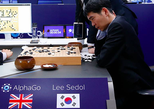
The most popular application for CNNs in the recent times has been Image Analysis, but many researchers have also found other interesting and exciting ways to use them: from winning Go matches against human players([7], a related video [8]) to an innovative application in discovering new drugs by training over large quantities of molecular structure data of organic compounds[9].

Motivation

A first question to answer with CNNs is why are they called Convolutional in the first place.

Convolution is a mathematical concept used heavily in Digital Signal Processing when dealing with signals that take the form of a time series. In lay terms, convolution is a mechanism to combine or “blend”[10] two functions of time³ in a coherent manner. It can be mathematically described as follows:

For a discrete domain of one variable:

For a discrete domain of two variables:

²A point to note here is the improvement is, in fact, modest. Classification accuracies greater than or equal to 99% on MNIST have been achieved using non-neural methods as well, such as K-Nearest Neighbours (KNN) or Support Vector Machines (SVM). For a list of ML methods applied and the respective classification accuracies attained, please refer to this[11] table.

³Or, for that matter, of another parameter.

Eq. 2 is perhaps more descriptive of what convolution truly is: a summation of pointwise products of function values, subject to traversal.

Though conventionally called as such, the operation performed on image inputs with CNNs is not strictly convolution, but rather a slightly modified variant called cross-correlation[10], in which one of the inputs is time-reversed:

CNN Concepts

CNNs have an associated terminology and a set of concepts that is unique to them, and that sets them apart from other types of neural network architectures. The main ones are explained as follows:

Input/Output Volumes

CNNs are usually applied to image data. Every image is a matrix of pixel values. The range of values that can be encoded in each pixel depends upon its bit size. Most commonly, we have 8 bit or 1 Byte-sized pixels. Thus the possible range of values a single pixel can represent is [0, 255]. However, with coloured images, particularly RGB (Red, Green, Blue)-based images, the presence of separate colour channels (3 in the case of RGB images) introduces an additional ‘depth’ field to the data, making the input 3-dimensional. Hence, for a given RGB image of size, say 255×255 (Width x Height) pixels, we’ll have 3 matrices associated with each image, one for each of the colour channels. Thus the image in it’s entirety, constitutes a 3-dimensional structure called the Input Volume (255x255x3).

Figure 1: The cross-section of an input volume of size: 4 x 4 x 3. It comprises of the 3 Colour channel matrices of the input image.

Features

Just as its literal meaning implies, a feature is a distinct and useful observation or pattern obtained from the input data that aids in performing the desired image analysis. The CNN learns the features from the input images. Typically, they emerge repeatedly from the data to gain prominence. As an example, when performing Face Detection, the fact that every human face has a pair of eyes will be treated as a feature by the system, that will be detected and learned by the distinct layers. In generic object classification, the edge contours of the objects serve as the features.

Filters (Convolution Kernels)

A filter (or kernel) is an integral component of the layered architecture.

Generally, it refers to an operator applied to the entirety of the image such that it transforms the information encoded in the pixels. In practice, however, a kernel is a smaller-sized matrix in comparison to the input dimensions of the image, that consists of real valued entries.

The kernels are then convolved with the input volume to obtain so-called ‘activation maps’. Activation maps indicate ‘activated’ regions, i.e. regions where features specific to the kernel have been detected in the input. The real values of the kernel matrix change with each learning iteration over the training set, indicating that the network is learning to identify which regions are of significance for extracting features from the data.

Kernel Operations Detailed

The exact procedure for convolving a Kernel (say, of size 16 x 16) with the input volume (a 256 x 256 x 3 sized RGB image in our case) involves taking patches from the input image of size equal to that of the kernel (16 x 16), and convolving (or calculating the dot product) between the values in the patch and those in the kernel matrix.

The convolved value obtained by summing the resultant terms from the dot product forms a single entry in the activation matrix. The patch selection is then slided (towards the right, or downwards when the boundary of the matrix is reached) by a certain amount called the ‘stride’ value, and the process is repeated till the entire input image has been processed. The process is carried out for all colour channels. For normalization purposes, we divide the calculated value of the activation matrix by the sum of values in the kernel matrix.

The process is demonstrated in Figure 2, using a toy example consisting of a 3-channel 4×4-pixels input image and a 3×3 kernel matrix.  Note that:

• pixels are numbered from 1 in the example;
• the values in the activation map are normalized to ensure the same intensity range between the input volume and the output volume. Hence, for normalization, we divide the calculated value for the ‘red’ channel by 2 (the sum of values in the kernel matrix);
• we assume the same kernel matrix for all the three channels, but it is possible to have a separate kernel matrix for each colour channel;
• for a more detailed and intuitive explanation of the convolution operation, you can refer to the excellent blog-posts by Chris Olah[12] and by Tim Dettmers[13].

Figure 2: The convolution value is calculated by taking the dot product of the corresponding values in the Kernel and the channel matrices. The current path is indicated by the red-coloured, bold outline in the Input Image volume. Here, the entry in the activation matrix is calculated as:

Receptive Field

It is impractical to connect all neurons with all possible regions of the input volume. It would lead to too many weights to train, and produce too high a computational complexity. Thus, instead of connecting each neuron to all possible pixels, we specify a 2 dimensional region called the ‘receptive field[14]’ (say of size 5×5 units) extending to the entire depth of the input (5x5x3 for a 3 colour channel input), within which the encompassed pixels are fully connected to the neural network’s input layer. It’s over these small regions that the network layer cross-sections (each consisting of several neurons (called ‘depth columns’)) operate and produce the activation map.

Zero-Padding

Zero-padding refers to the process of symmetrically adding zeroes to the input matrix. It’s a commonly used modification that allows the size of the input to be adjusted to our requirement. It is mostly used in designing the CNN layers when the dimensions of the input volume need to be preserved in the output volume.

Figure 3: A zero-padded 4 x 4 matrix becomes a 6 x 6 matrix.

Hyperparameters

In CNNs, the properties pertaining to the structure of layers and neurons, such spatial arrangement and receptive field values, are called hyperparameters. Hyperparameters uniquely specify layers. The main CNN hyperparameters are receptive field (R), zero-padding (P), the input volume dimensions (Width x Height x Depth, or W x H x D ) and stride length (S).

The CNN Architecture

Now that we are familiar with the CNN terminology, let’s go on ahead and study the CNN architecture in detail.

The architecture of a typical CNN is composed of multiple layers where each layer performs a specific function of transforming its input into a useful representation. There are 3 major types of layers that are commonly observed in complex neural network architectures:

Convolutional Layer
Also referred to as Conv. layer, it forms the basis of the CNN and performs the core operations of training and consequently firing the neurons of the network. It performs the convolution operation over the input volume as specified in the previous section, and consists of a 3-dimensional arrangement of neurons (a stack of 2-dimensional layers of neurons, one for each channel depth).

Figure 4: A 3-D representation of the Convolutional layer with 3 x 3 x 4 = 36 neurons.

Each neuron is connected to a certain region of the input volume called the receptive field (explained in the previous section). For example, for an input image of dimensions 28x28x3, if the receptive field is 5 x 5, then each neuron in the Conv. layer is connected to a region of 5x5x3 (the region always comprises the entire depth of the input, i.e. all the channel matrices) in the input volume. Hence each neuron will have 75 weighted inputs. For a particular value of R (receptive field), we have a cross-section of neurons entirely dedicated to taking inputs from this region. Such a cross-section is called a ‘depth column’. It extends to the entire depth of the Conv. layer.

For optimized Conv. layer implementations, we may use a Shared Weights model that reduces the number of unique weights to train and consequently the matrix calculations to be performed per layer. In this model, each ‘depth slice’ or a single 2-dimensional layer of neurons in the Conv architecture all share the same weights. The caveat with parameter sharing is that it doesn’t work well with images that encompass a spatially centered structure (such as face images), and in applications where we want the distinct features of the image to be detected in spatially different locations of the layer.

Figure 5: Concept of Receptive Field.

We must keep in mind though that the network operates in the same way that a feed-forward network would: the weights in the Conv layers are trained and updated in each learning iteration using a Back-propagation algorithm extended to be applicable to 3-dimensional arrangements of neurons.

The ReLu (Rectified Linear Unit) Layer

ReLu refers to the Rectifier Unit, the most commonly deployed activation function for the outputs of the CNN neurons. Mathematically, it’s described as:

Unfortunately, the ReLu function is not differentiable at the origin, which makes it hard to use with backpropagation training. Instead, a smoothed version called the Softplus function is used in practice:

The derivative of the softplus function is the sigmoid function, as mentioned in a prior blog post.

The Pooling Layer

The pooling layer is usually placed after the Convolutional layer. Its primary utility lies in reducing the spatial dimensions (Width x Height) of the Input Volume for the next Convolutional Layer. It does not affect the depth dimension of the Volume.  

The operation performed by this layer is also called ‘down-sampling’, as the reduction of size leads to loss of information as well. However, such a loss is beneficial for the network for two reasons:

1. the decrease in size leads to less computational overhead for the upcoming layers of the network;
2. it work against over-fitting.

Much like the convolution operation performed above, the pooling layer takes a sliding window or a certain region that is moved in stride across the input transforming the values into representative values. The transformation is either performed by taking the maximum value from the values observable in the window (called ‘max pooling’), or by taking the average of the values. Max pooling has been favoured over others due to its better performance characteristics.

The operation is performed for each depth slice. For example, if the input is a volume of size 4x4x3, and the sliding window is of size 2×2, then for each color channel, the values will be down-sampled to their representative maximum value if we perform the max pooling operation.

No new parameters are introduced in the matrix by this operation. The operation can be thought of as applying a function over input values, taking fixed sized portions at a time, with the size, modifiable as a parameter. Pooling is optional in CNNs, and many architectures do not perform pooling operations.

Figure 6: The Max-Pooling operation can be observed in sub-figures (i), (ii) and (iii) that max-pools the 3 colour channels for an example input volume for the pooling layer. The operation uses a stride value of [2, 2]. The dark and red boundary regions describe the window movement. Sub-figure (iv) shows the operation applied for a stride value of [1,1], resulting in a 3×3 matrix Here we observe overlap between regions.

The Fully Connected Layer

The Fully Connected layer is configured exactly the way its name implies: it is fully connected with the output of the previous layer. Fully-connected layers are typically used in the last stages of the CNN to connect to the output layer and construct the desired number of outputs.

CNN Design Principles

Given the aforementioned building blocks, the last detail before implementing a CNN is to specify its design end to end, and to decide on the layer dimensions of the Convolutional layers.

A quick and dirty empirical formula[15] for calculating the spatial dimensions of the Convolutional Layer as a function of the input volume size and the hyperparameters we discussed before can be written as follows:

For each (ith) dimension of the input volume, pick:

where is the (ith) input dimension, R is the receptive field value, P is the padding value, and S is the value of the stride. Note that the formula does not rely on the depth of the input.

To better understand better how it works, let’s consider the following example:

1. Let the dimensions of the input volume be 288x288x3, the stride value be 2 (both along horizontal and vertical directions).
2. Now, since W_In=288 and S = 2, (2.P – R) must be an even integer for the calculated value to be an integer. If we set the padding to 0 and R = 4, we get W_Out=(288-4+2.0)/2+1 =284/2 + 1 = 143. As the spatial dimensions are symmetrical (same value for width and height), the output dimensions are going to be: 143 x 143 x K, where K is the depth of the layer. K can be set to any value, with increasing values for every Conv. layer added. For larger networks values of 512 are common.
3. The output volume from a Conv. layer either has the same dimensions as that of the Conv. layer (143x143x2 for the example considered above), or the same as that of the input volume (288x288x3 for the example above).

The generic arrangement of layers can thus be summarized as follows[15]:

Where N usually takes values between 0 and 3, M >= 0 and K∈[0,3).

The expression indicates multiple layers, with or without per layer-Pooling. The final layer is the fully-connected output layer. See [8] for more case-studies of CNN architectures, as well as a detailed discussion of layers and hyper-parameters.  

Conclusion

CNNs showcase the awesome levels of control over performance that can be achieved by making effective use of theoretical and mathematical insights. Many real world problems are being efficiently tackled using CNNs, and MNIST represents a simple, “Hello World”-type use-case of this technique. More complex problems such as object and image recognition require the use of deep neural networks with millions of parameters to obtain state-of-the-art results. CIFAR-10 is a good problem to solve in this domain, and it was first solved by Alex Krizhevsky et al.[16] in 2009. You can read through the technical report and try and grasp the approach before making way to the TensorFlow tutorial that solves the same problem[17].

Furthermore, applications are not limited to computer vision. The most recent win of Google’s AlphaGo Project over Lee Sedol in the Go game series relied on a CNN at its core. The self-driving cars which, in the coming years, will arguably become a regular sight on our streets, rely on CNNs for steering[18]. Google even held an art-show[19] for imagery created by its DeepDream project that showcased beautiful works of art created by visualizing the transformations of the network!

Thus a Machine Learning researcher or engineer in today’s world can rejoice at the technological melange of techniques at her disposal, among which an in-depth understanding of CNNs is both indispensable and empowering.

References

[1] Hopfield, John J. “Neural networks and physical systems with emergent collective computational abilities.” Proceedings of the national academy of sciences 79.8 (1982): 2554-2558.[http://www.pnas.org/content/79/8/2554.abstract]

[2]  Rumelhart, D. E., Hinton, G. E., and Williams, R. J. (1986). Learning representations by back-propagating errors. Nature, 323, 533–536.[http://www.iro.umontreal.ca/~vincentp/ift3395/lectures/backprop_old.pdf]

[3]   Andrey Kurenkov, “A brief History of Neural Nets and Deep Learning”.[http://www.andreykurenkov.com/writing/a-brief-history-of-neural-nets-and-deep-learning/]

[4]  LeCun, Yann, et al. “Gradient-based learning applied to document recognition.” Proceedings of the IEEE 86.11 (1998): 2278-2324.

[5] The MNIST database of handwritten digits

[6] Hubel, David H., and Torsten N. Wiesel. “Receptive fields and functional architecture of monkey striate cortex.” The Journal of physiology 195.1 (1968): 215-243.

[7] Alpha Go video by Nature.                                             [http://www.nature.com/news/google-ai-algorithm-masters-ancient-game-of-go-1.19234]

[8] Clark, Christopher, and Amos Storkey. “Teaching deep convolutional neural networks to play go.” arXiv preprint arXiv:1412.3409 (2014).[http://arxiv.org/pdf/1412.3409.pdf]

[9] Wallach, Izhar, Michael Dzamba, and Abraham Heifets. “AtomNet: A Deep Convolutional Neural Network for Bioactivity Prediction in Structure-based Drug Discovery.” arXiv preprint arXiv:1510.02855 (2015).

[http://arxiv.org/pdf/1510.02855.pdf]

[10] Weisstein, Eric W. “Convolution.” From MathWorld — A Wolfram Web Resource. [http://mathworld.wolfram.com/Convolution.html]

[11] Table of classification accuracies attained over MNIST. [https://en.wikipedia.org/wiki/MNIST_database#Performance]

[12] Chris Olah, “Understanding Convolutions”.                           [http://colah.github.io/posts/2014-07-Understanding-Convolutions/]

[13] Tim Dettmers, “Understanding Convolution In Deep Learning”.[http://timdettmers.com/2015/03/26/convolution-deep-learning/]

[14] TensorFlow Documentation: Convolution [https://www.tensorflow.org/versions/r0.7/api_docs/python/nn.html#convolution]

[15] Andrej Karpathy, “CS231n: Convolutional Neural Networks for Visual Recognition” [http://cs231n.github.io/convolutional-networks/]

[16] Krizhevsky, Alex, and Geoffrey Hinton. “Learning multiple layers of features from tiny images.” (2009).[http://www.cs.toronto.edu/~kriz/learning-features-2009-TR.pdf]

[17] TensorFlow: Convolutional Networks.[https://www.tensorflow.org/versions/r0.7/tutorials/deep_cnn/index.html#cifar-10-model]

[18] Google Deepmind’s AlphaGo: How it works.       [https://www.tastehit.com/blog/google-deepmind-alphago-how-it-works/]

[19] An Empirical Evaluation of Deep Learning on Highway Driving.[http://arxiv.org/pdf/1504.01716.pdf]

[20] Inside Google’s First DeepDream Art Project. [http://www.fastcodesign.com/3057368/inside-googles-first-deepdream-art-show/11]