Recommended Books - UC Berkeley Statistics Graduate Student Association
Machine Learning/course 2018. 2. 26. 15:22http://sgsa.berkeley.edu/current-students/recommended-books
Applied Statistics
Categorical Data
- ''Categorical Data Analysis'' by Alan Agresti
- Well-written, go-to reference for all things involving categorical data.
Linear models
- ''Generalized Linear Models'' by McCullagh and Nelder
- Theoretical take on GLMs. Does not have a lot of concrete data examples.
- ''Statistical Models'' by David A. Freedman
- ...Berkeley classic!
- ''Linear Models with R'' by Julian Faraway
- Undergraduate-level textbook, has been used previously as a textbook for Stat 151A. Appropriate for beginners to R who would like to learn how to use linear models in practice. Does not cover GLMs.
Experimental Design
- ''Design of Comparative Experiments'' by RA Bailey
- Classic, approachable text, free for download here
Machine Learning
- ''The Elements of Statistical Learning'' by Hastie, Tibshirani, and Friedman.
- Comprehensive but superficial coverage of all modern machine learning techniques for handling data. Introduces PCA, EM algorithm, k-means/hierarchical clustering, boosting, classification and regression trees, random forest, neural networks, etc. ...the list goes on. Download the book here.
- ''Computer Age Statistical Inference: Algorithms, Evidence, and Data Science'' by Hastie and Efron.
- ''Pattern Recognition and Machine Learning'' by Bishop.
- ''Bayesian Reasoning and Machine Learning'' by Barber. Available online.
- ''Probabilistic Graphical Models'' by Koller and Friedman.
Theoretical Statistics
- ''Theoretical Statistics: Topics for a Core Course'' by Keener
- The primary text for Stat 210A. Download from SpringerLink.
- ''Theory of Point Estimation'' by Lehmann and Casella
- A good reference for Stat 210A.
- ''Testing Statistical Hypotheses'' by Lehmann and Romano
- A good reference for Stat 210A.
- ''Empirical Processes in M-Estimation'' by van de Geer
- Some students find this helpful to supplement the material in 210B.
Probability
Undergraduate Level Probability
- ''Probability'' by Pitman
- What the majority of Berkeley undergraduates use to learn probability.
- ''Introduction to Probability Theory'' by Hoel, Port and Stone
- This text is more mathematically inclined than Pitman's, and more concise, but not as good at teaching probabilistic thinking.
- ''Probability and Computing'' by Upfal and Mitzenmacher
- What students in EECS use to learn about randomized algorithms and applied probability.
Measure Theoretic Probability
- ''Probability: Theory and Examples'' by Durrett
- This is the standard text for learning measure theoretic probability. Its style of presentation can be confusing at times, but the aim is to present the material in a manner that emphasizes understanding rather than mathematical clarity. It has become the standard text in Stat 205A and Stat 205B for good reason. Online here.
- ''Foundations of Modern Probability'' by Olav Kallenberg
- This epic tome is the ultimate research level reference for fundamental probability. It starts from scratch, building up the appropriate measure theory and then going through all the material found in 205A and 205B before powering on through to stochastic calculus and a variety of other specialized topics. The author put much effort into making every proof as concise as possible, and thus the reader must put in a similar amount of effort to understand the proofs. This might sound daunting, but the rewards are great. This book has sometimes been used as the text for 205A.
- ''Probability and Measure'' by Billingsley
- This text is often a useful supplement for students taking 205 who have not previously done measure theory. Download here.
- ''Probability with Martingales'' by David Williams
- This delightful and entertaining book is the fastest way to learn measure theoretic probability, but far from the most thorough. A great way to learn the essentials.
Stochastic Calculus
Stochastic Calculus is an advanced topic that interested students can learn by themselves or in a reading group. There are three classic texts:
- ''Continuous Martingales and Brownian Motion'' by Revuz and Yor
- ''Diffusions, Markov Processes and Martingales (Volumes 1 and 2)'' by Rogers and Williams
- ''Brownian Motion and Stochastic Calculus'' by Karatzas and Shreve
Random Walk and Markov Chains
These are indispensable tools of probability. Some nice references are
- ''Markov Chain and Mixing Times'' by Levin, Peres and Wilmer. Online here.
- ''Markov Chains'' by Norris
- Starting with elementary examples, this book gives very good hints on how to think about Markov Chains.
- ''Continuous time Markov Processes'' by Liggett
- A theoretical perspective on this important topic in stochastic processes. The text uses Brownian motion as the motivating example.
Mathematics
Convex Optimization
- ''Convex Optimization'' by Boyd and Vandenberghe. : You can download the book here
- ''Introductory Lectures on Convex Optimization'' by Nesterov.
Linear Algebra
- ''The Matrix Cookbook'' by Petersen and Pedersen: ''Matrix identities, relations and approximations. A desktop reference for quick overview of mathematics of matrices.'' Download here.
- ''Matrix Analysis'' and ''Topics in Matrix Analysis'' by Horn and Johnson
- Second book is more advanced than the first. Everything you need to know about matrix analysis.
Convex Analysis
- ''A course in Convexity'' by Barvinok.
- A great book for self study and reference. It starts with the basis of convex analysis, then moves on to duality, Krein-Millman theorem, duality, concentration of measure, ellipsoid method and ends with Minkowski bodies, lattices and integer programming. Fairly theoretical and has many fun exercises.
Measure Theory
- Real Analysis and Probability - Dudley
- Very comprehensive.
- Probability and Measure Theory - Ash
- Nice and easy to digest. Good as companion for 205A
Combinatorics
- ''Enumerative Combinatorics Vol I and II'' - Richard Stanley.
- There's also a course on combinatorics this semester in the math department called Math249: Algebraic Combinatorics. Despite the scary "algebraic" prefix it's really fun. Download here.
Computational Biology
- ''Statistical Methods in Bioinformatics'' by Ewens and Grant
- Great overview of sequencing technology for the unacquainted.
- ''Computational Genome Analysis: An Introduction'' by Deonier, Tavare, and Waterman
- Great R code examples from computational biology. Discusses the basics, such as the greedy algorithm, etc.
Population Genetics
- ''Probability Models for DNA Sequence Evolution'' by Durrett
- ''Mathematical Population Genetics'' by Ewens
Computer Science
Numerical Analysis
- Numerical Analysis by Burden and Faires
- This book is a good overview of numerical computation methods for everything you'd need to know about implementing most computational methods you'll run into in statistics. It is filled with pseudo-code but does use Maple as it's exemplary language sometimes. It has been a great resource for the Computational Statistics courses (243/244). Depending on what happens with this course, this may be a good place to look when you're lost in computation.
Algorithms
- ''Introduction to Algorithms'', Third Edition, by Cormen, Leiserson, Rivest, and Stein.
- Amazon
- Google Books
- MIT OpenCourseWare 6.046J / 18.410J ''Introduction to Algorithms'' (SMA 5503) was taught by one of the authors, Prof. Charles Leiserson, in 2005. This is an undergraduate course and this book was used as the textbook
- ''Algorithm Design'', by Jon Kleinberg and Éva Tardos.
'Machine Learning > course' 카테고리의 다른 글
| 머신러닝 공부 순서, 방법 및 강의 정리(HowUse 곰씨네) (0) | 2019.01.22 |
|---|---|
| 머신러닝 공부순서 (0) | 2018.12.03 |
| 통계 추천 동영상강좌 (0) | 2017.12.16 |
| Pattern Recognition and Machine Learning 책 2장 식(2.117)까지 정리한 노트입니다. (0) | 2017.11.08 |
| 앤드류 교수의 코세라 강의를 정주행 후 영상 슬라이드를 정리하여 (0) | 2017.08.03 |


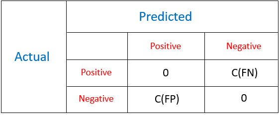 Cost Matrix
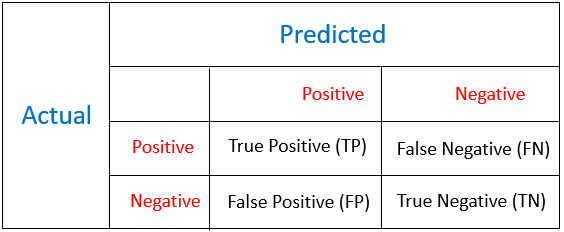 Confusion Matrix