'Deep Learning'에 해당되는 글 593건

  1. 2017.02.28 Understanding, generalisation, and transfer learning in deep neural networks
  2. 2017.02.08 Machine Learning Top 10 Articles for the Past Year (v.2017)
  3. 2017.02.07 Windows 에서 Tensorflow GPU를 사용하는 방법
  4. 2017.02.07 윈도우 10 + 케라스 (tensorflow backend) + 아나콘다로 <케라스 설치하기>
  5. 2017.02.02 라온피플 머신 러닝(Machine Learning) - Class
  6. 2017.02.02 Fully Convolutional Networks (FCNs) for Image Segmentation
  7. 2017.01.31 Intro to Machine Learning using Tensorflow – Part 1
  8. 2017.01.31 Machine Learning Top 10 Articles for the Past Year (v.2017)
  9. 2017.01.31 무료 e-러닝 강좌 머신러닝을 이용한 주식 트레이딩
  10. 2017.01.23 Visualizing parts of Convolutional Neural Networks using Keras and Cats
  11. 2017.01.23 Introduction to Deep Learning for Computer Vision
  12. 2017.01.21 Learn TensorFlow and deep learning, without a Ph.D. 동영상강의 슬라이드
  13. 2017.01.19 YouTube에서 'How to Do Linear Regression the Right Way [LIVE]' 보기
  14. 2017.01.19 sequence-to-sequence 모델인 "Pointer Networks 구현
  15. 2017.01.18 Linear Regression / Bias-Variance Decomposition
  16. 2017.01.18 Implementation of Grad CAM in tensorflow
  17. 2017.01.17 GPU-accelerated Theano & Keras on Windows 10 native
  18. 2017.01.13 Recognizing Traffic Lights With Deep LearningHow I learned deep learning in 10 weeks and won $5,000
  19. 2017.01.12 YouTube에서 'How to Install Tensorflow on Windows10 with GPU support' 보기
  20. 2017.01.12 Installing Theano in Windows 7 64-bit
  21. 2017.01.11 DeepLab-ResNet-TensorFlow
  22. 2017.01.10 Deep Learning in Action
  23. 2017.01.10 Up and running with Theano (GPU) + PyCUDA on Windows
  24. 2017.01.10 If CNN denoises images knowing content, it gets better results. Simple idea, great paper! https://arxiv.org/abs/1701.01698 Deep Class Aware Denoising
  25. 2017.01.09 딥러닝을 이용한 숫자 이미지 인식 #1/2-학습
  26. 2017.01.08 마코프에 이어서 강화학습에 대해서는 아래 영상이 가장 쉬웠습니다.
  27. 2017.01.06 Keras, Theano and TensorFlow on Windows and Linux | GetToCode
  28. 2017.01.05 YouTube에서 'Installing CPU and GPU TensorFlow on Windows' 보기
  29. 2017.01.05 YouTube에서 'how to natively install tensorflow on windows' 보기
  30. 2017.01.03 Modern optimization methods from gradient descent family are the key to the majority of modern data-driven solutions. Sebastian Ruder does the great job explaining the modern optimization methods.

Understanding, generalisation, and transfer learning in deep neural networks | the morning paper
https://blog.acolyer.org/2017/02/27/understanding-generalisation-and-transfer-learning-in-deep-neural-networks/

Menu

the morning paper
an interesting/influential/important paper from the world of CS every weekday morning, as selected by Adrian Colyer
Understanding, generalisation, and transfer learning in deep neural networks
This is the first in a series of posts looking at the ‘top 100 awesome deep learning papers.’ Deviating from the normal one-paper-per-day format, I’ll take the papers mostly in their groupings as found in the list (with some subdivision, plus a few extras thrown in) – thus we’ll be looking at multiple papers each day. The papers in today’s selection all shed light on what it is that DNNs (mostly CNNs) are really learning when trained. Since one way of understanding what a DNN has truly learned is to see how well the trained networks (or subsets of them) can perform on new tasks, we’ll also learn a lot about generalization, and what we learn can help us to define better models that take advantage of transfer learning.

The six papers we’ll look at today are:

Visualizing and understanding convolutional networks, Zeller & Fergus 2013
DeCAF: A deep convolutional activation feature for generic visual recognition, Donahue et al., 2014
CNN features off-the-shelf: an astounding baseline for recognition, Razavian et al., 2014
How transferable are features in deep neural networks? Yosinski et al., 2014
Learning and transferring mid-level image representations using convolutional neural networks, Oquab et al., 2014
Distilling the knowledge in a neural network, Hinton et al., 2015
I’ve done my best to distill the knowledge in these papers too, but inevitably this post is going to be a little longer than my normal target length! You might need one-and-a-half cups of coffee for this one ;).

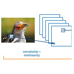
Visualising and understanding convolutional networks

Convolutional neural networks (convnets) have demonstrated excellent performance at tasks such as hand-written digit classification and face detection… Despite this encouraging progress, there is still little insight into the internal operation and behavior of these complex models, or how they achieve such good performance. From a scientific standpoint, this is deeply unsatisfactory.

If we’re going to understand what a convnet is doing, we need some way to map the feature activity in intermediate layers back into the input pixel space (we’re working with Convnets trained on the ImageNet dataset here). Zeiler and Fergus use a clever construction that they call a deconvnet that uses the same components as the convnet to be decoded, but in reverse order. Some of the convnet components need to be augmented slightly to capture additional information that helps in the reversing process. (It’s a little reminiscent of the data flow provenance work that we looked at earlier this year.)

Here’s an example with the standard convnet on the right-hand side, and the deconvnet layers added on the left-hand side.


Now that we can project from any layer back onto pixels, we can get a peek into what they seem to be learning. This leads to now-familiar pictures such as this:


Note in the above how layer 2 responds to corners and edge/colour combinations, layer 3 seems to capture similar textures, layer 4 is more class-specific (e.g. dog faces), and layer 5 shows entire objects with significant pose variation. Using these visualisations and looking at how they change over time during training it is also possible to see lower layers converging within relatively few epochs, whereas upper layers take considerably longer to converge. Small transformations in the input image have a big effect on lower layers, but lesser impact in higher layers.

The understanding gleaned from inspecting these visualisations proved to be a helpful tool for improving the underlying models too. For example, a 2nd layer visualization showed aliasing artefacts caused by a large stride size, reducing the stride size gave an increase in classification performance.

Experiments with model structure showed that having a minimum depth to the network, rather than any one specific section in the overall model, is vital to model performance.

DeCAF: A deep convolutional activation feature for generic visual recognition

Many visual recognition challenges have data sets with comparatively few examples. In DeCAF, the authors explore whether a convolutional network trained on ImageNet (a large dataset) can be generalised to other tasks where less data is available:

Our model can either be considered as a deep architecture for transfer learning based on a supervised pre-training phase, or simply as a new visual feature DeCAF defined by the convolutional network weights learned on a set of pre-defined object recognition tasks.

After training deep a convolutional model (using Krizhevskey et al.’s competition winning 2012 architecture), features are extracted from the resulting model and used as inputs to generic vision tasks. Success in those task would indicate that the convolutional network is learning generically useful features of images (in much the same way that word embeddings learn features of words).

Let DeCAFn be the activations of the nth hidden layer of the CNN. DeCAF7 is the final hidden layer just before propagating through the last fully connected layer to produce class predictions. All of the weights from the CNN up to the layer under test are frozen, and either a logistic regression or support vector machine is trained using the CNN features as input.

On the Caltech-101 dataset the DeCAF6 + SVM outperformed the previous best state of the art (a method with a combination of five traditional hand-engineered image features)!

The Office dataset contains product images from amazon.com, as well as images taken in office environments using webcams and DSLRs. DeCAF features were shown to be robust to resolution changes (webcam vs DSLR), providing not only better within category clustering, but also was able to cluster same category instances across domains. DeCAF + SVM again dramatically outperformed the baseline SURF features available with the Office dataset.

For sub-category recognition (e.g. distinguishing between lots of different bird types in the Caltech-UCSD birds dataset) DeCAF6 with simple logistic regression again obtained a significant increase over existing approaches: “To the best of our knowledge, this is the best accuracy reported so far in the literature.”

And finally, for scene recognition tasks, DeCAF + logistic regression on the SUN-397 large-scale scene recognition database also outperformed the current state-of-the-art.

Convolution neural networks trained on large image sets were therefore forcefully demonstrated to learn features with sufficient representational power and generalization ability to perform at state-of-the-art levels on a wide variety of image-based tasks. It’s the beginning of the end of hand-engineered features, and welcome to the era of deep-learned features.

The ability of a visual recognition system to achieve high classification accuracy on tasks with sparse labeled data has proven to be an elusive goal in computer vision research, but our multi-task deep learning framework and fast open-source implementation are significant steps in this direction.

CNN features off-the-shelf: an astounding baseline for recognition

CNN features off the shelf further reinforces that we can learn general features useful for image-based tasks, and apply them very successfully in new domains. This time the baseline features are taken from a trained convolutional neural network model called Overfeat, which has been optimized for object image classification in ILSVRC. Then for a variety of tasks, instead of using state-of-art image processing pipelines, the authors simply take the features from the CNN representation, and bolt on an SVM. Sounds familiar?


The tasks undertaken progress from quite close to the original classification task, to more and more demanding (i.e. distant tasks). At every step of the way, the CNN features prove their worth!

Step 1: Object and scene recognition
The Pascal VOC 2007 dataset has ~10,000 images of 20 classes of animals, and is considered more challenging than ILSVRC. Applying the Overfeat CNN features to this dataset resulted in a model outperforming all previous efforts “by a significant margin.” The following chart shows how classification performance improves depending on the level from the original CNN that is chosen as the input to the final SVM:


For scene recognition, the MIT-67 indoor scene dataset has 15,620 images of 67 indoor scene classes. The CNN + SVM model significantly outperformed a majority of the baseline models and just edges a state-of-the-art award by 0.1% accuracy over the previous best AlexConvNet model (also a CNN).

Step 2: Fine-grained recognition
Here we’re back with birds (Caltech UCSD 200-2011 dataset) and also flowers (Oxford 102 flowers dataset). Can the more generic OverFeat features pick up potentially subtle differences between the very similar classes? On the birds dataset the model gets very close to the state of the art (also a CNN), and beats all other baselines. On the flowers dataset, the CNN+SVM model outperforms the previous state-of-the-art.

Step 3: Attribute detection
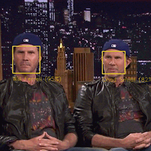
Have the OverFeat features encoded something about the semantic properties of people and objects? The H3D dataset defines 9 attributes for person images (for example, ‘has glasses,’ and ‘is male.’). The UIUC 64 dataset has attributes for objects (e.g., ‘is 2D boxy’, ‘has head’, ‘is furry’). The CNN-SVM achieves state of the art on UIUC 64, and beat several existing models on H3D.

Step 4: Instance retrieval
What about trying the CNN-SVM model on instance retrieval problems? This is a domain where the state-of-the-art using highly optimized engineered vectors and mid-level features. Against methods that do not incorporate 3D geometric constraints (which do better), the CNN features proved very competitive on building and holiday datasets.

What have we learned?
It’s all about the features! SIFT and HOG descriptors produced big performance gains a decade ago and now deep convolutional features are providing a similar breakthrough for recognition. Thus, applying the well-established computer vision procedures on CNN representations should potentially push the reported results even further. In any case, if you develop any new algorithm for a recognition task, it must be compared against the strong baseline of generic deep features + simple classifier.

How transferable are features in deep neural networks?

The previous papers mostly focused on taking the higher layers from the pre-trained CNNs as input features. In ‘How transferable are features in deep neural networks’ the authors systematically explore the generality of the features learned at each layer – and as we’ve seen, to the extent that features at a given layer are general, we’ll be able to use them for transfer learning.

The usual transfer learning approach is to train a base network and then copy its first n layers to the the first n layers of a target network. The remaining layers of the target network are then randomly initialized and trained toward the target task. One can choose to back-propagate the errors from the new task into the base (copied) features to fine-tune them to the new task, or the transferred feature layers can be left frozen…

The experiment setup is really neat. Take an 8-layer CNN model, and split the 1000 ImageNet classes into two groups (so that each contains approximately half the data or 645,000 examples). Train one instance of the model on half A, and call it baseA. Train another instance of the model on half B, and call it baseB. Starting with baseA, we can define seven starter networks, A1 through A7, that copy the first 1 through 7 layers from baseA respectively (and of course we can do the same from baseB to give B1 through B7). Say we’re interested in exploring how well features learned at layer 3 transfer. We can construct the following four networks:

B3B – the first 3 layers are copied from baseB and frozen. The remaining five higher layers are initialized randomly and we train on task B as a control. (The authors call this a ‘selfer’ network)
A3B – the first 3 layers are copied from baseA and frozen. The remaining five layers are initialized randomly as before, and trained on task B. If A3B performs as well as B3B, we have evidence that the first three layers are general.
B3B+, like B3B but the first three layers are subsequently fine-tuned during training.
A3B+, like A3B but the first three layers are subsequently fine-tuned during training.


Repeat this process for all layers 1..7. Running these experiments leads to the following results:


Looking at the dark blue dots first (BnB), we see an interesting phenomenon. When freezing early layers and then retraining the later layers towards the same task, the resulting performance is very close to baseB. But layers 3,4,5, and 6 (especially 4 and 5) show significantly worse performance:

This performance drop is evidence that the original network contained fragile co-adapted features on successive layers.

As we get closer to the final layers, performance is restored as it seems there is less to learn… “To our knowledge it has not been previously observed in the literature that such optimization difficulties may be worse in the middle of a network than near the bottom or top.”

Note that the light blue dots (BnB+), where we allow fine-tuning, restore full performance.

The red dots show the transfer learning results. Starting with the frozen base version (dark red, AnB), we see strong transference in layers 1 and 2, and only a slight drop in layer 3, indicating that the learned features are general. Through layers 4-7 though we see a significant drop in performance.

Thanks to the BnB points, we can tell that this drop is from a combination of two separate effects: the drop from lost co-adaptation and the drop from features that are less and less general.

Finally let’s look at the light red AnB+ points. These do better than the baseline! Surprised? Even when the dataset is large, transferring features seems to boost generalization performance. Keeping anywhere from one to seven layers seems to infer some benefit (average boost 1.6%) so the effect is seen everywhere. One way that I think about this is that the transferred layers had a chance to learn from different images that the selfer networks never see – thus they have a better chance of learning better generalizations.

The short summary – transfers can improve generalization performance. Two issues impact how well transfer occurs: fragile co-adaptation of middle layers, and specialisation of higher layers.

Learning and transferring mid-level image representations using convolutional neural networks

This paper uses the by-now familiar ‘train a CNN on ImageNet and extract features to transfer to other tasks approach, but also explores training techniques that can help to maximise the transfer benefits. Here’s the setup:


The target task for transfer learning is Pascal VOC object and action classification, “we wish to design a network that will output scores for target categories, or background if none of the categories are present in the image.” Transfer is achieved by removing the last fully-connected layer from the pre-trained network and adding an adaption layer formed of two fully-connected layers.

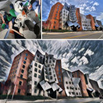
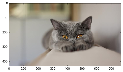
The source dataset (ImageNet) contains nice images of single centered objects. The target dataset (Pascal VOC) contains complex scenes with multiple target objects at various scales and background clutter:


The distributed of object orientations and sizes as well as, for example, their mutual occlusion patterns is very different between the two tasks. This issue has also been called “a dataset capture bias.” In addition, the target task may contain many other objects not present in the source task training data (“a negative bias”).

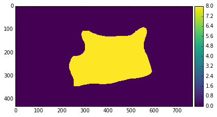
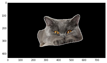
Here’s the new twist: to address these biases, the authors use a sliding window and extract around 500 square patches from each image by sampling on eight different scales using a regularly spaced grid and 50% or more overlap between neighbouring patches:


To label the patches in the resulting training data, the authors measure the overlap between the bounding box of a patch P and the ground truth bounding boxes of annotated objects in the image. If there is sufficient overlap with a given class, the patch is labelled as a positive training example for the class.

You shouldn’t be surprised at this point to learn that the resulting network achieves state of the art performance on Pascal VOC 2007 object recognition, and gets very close to the state of the art on Pascal VOC 2012. The authors also demonstrate that the network learns about the size and location of target objects within the image. For the Pascal VOC 2012 action recognition task, state of the art results were achieved by allowing fine-tuning of the copied layers during training.

Our work is part of the recent evidence that convolutional neural networks provide means to learn rich mid-level image features transferrable to a variety of visual recognition tasks.

Distilling the knowledge in a neural network

Let’s finish with something a little bit different: what can insects teach us about neural network training and design?

Many insects have a larval form that is optimized for extracting energy and nutrients from the environment and a completely different adult form that is optimized for the very different requirements of traveling and reproduction. In large-scale machine learning, we typically use very similar models for the training stage and the deployment stage despite their very different requirements.

What if we use large cumbersome models during training (e.g.,very deep networks, ensembles), so long as those models make it easier to extract structure from the training data, and then find a way to transfer or distill that the training model has learned into a a more compact form suitable for deployment? We want to cram as much of the knowledge as possible from the large model into the smaller one.

If the cumbersome model generalizes well because, for example, it is the average of a large ensemble of different models, a small model trained to generalize in the same way will typically do much better on test data than a small model that is trained in the normal way on the same training set as was used to train the ensemble.

How can we train the small model effectively though? By using the class probabilities produced by the cumbersome model as “soft targets” for training the small model. The large model has learned not just the target prediction class, but a probability distribution over all classes – and the relative probabilities of incorrect answers still contain a lot of valuable information. The essence of the idea is to train the small model to reproduce the probability distribution, not just the target output class.

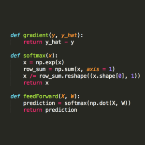
Neural networks typically produce class probabilities by using a “softmax” output layer that converts the logit, _zi_, computed for each class into a probability, _qi_, by comparing _zi_ with the other logits.

q_i = \frac{\exp(z_i/T)}{\sum_j{\exp(z_j/T)}}

where T is a temperature normally set to 1. A higher T value produces a softer probability distribution over classes. The cumbersome model is trained using a high temperature in its softmax, and the same high temperature is used when training the distilled model. When that model is deployed though, it uses a temperature of 1.

A ‘cumbersome’ large neural net with two hidden layers of 1200 rectified linear units trained on 60,000 training cases using dropouts to simulate training an ensemble of models sharing weights,achieved only 67 test errors. A smaller model network with 800 units in each layer and no regulalization saw 146 test errors. However, a distilled smaller network of the same size trained to match the soft targets from the large network achieved only 74 test errors.

In an Automatic Speech Recognition (ASR) test an ensemble of 10 models was distilled to a single model that performed almost as well. The results compare well to a very strong baseline model similar to that used by Android voice search.


A very nice use of the technique is in learning specialized models as part of an ensemble. Take a large data set (e.g. Google’s JFT image dataset with 100M images) and a large number of labels (15,000 in JFT): it’s likely there are several subsets of labels on which a general model gets confused. Using a clustering algorithm to find classes that are often predicted together, an ensemble is created with one generalist model, and many specialist models, one for each of the top k clusters. The specialist models are trained on data highly enriched in examples from the confusable subsets. The hope is that the resulting knowledge can be distilled back into a single large net, although the authors did not demonstrate that final step in the paper.

We have shown that distilling works very well for transferring knowledge from an ensemble or from a large highly regularized model into a smaller, distilled model…. [Furthermore,] we have shown that the performance of a single really big net that has been trained for a long time can be significantly improved by learning a large number of specialist nets, each of which learns to discriminate between the classes in a highly confusable cluster.

Understanding through counter-examples

Another interesting way of understanding what DNNs have learned, is through the discovery of counter-examples that confuse them. The ‘top 100 awesome deep learning papers‘ section on understanding, generalisation, and transfer learning (which we’ve been working through today) contains one paper along those lines. But this post is long enough already, and the subject is sufficiently interesting that I’d like to expand it with a few additional papers as well. So we’ll look at that tomorrow…

Share this:
TwitterLinkedIn3EmailPrint

Related
Distributed TensorFlow with MPI
With 4 comments
ImageNet Classification with Deep Convolutional Neural Networks
In "Machine Learning"
Matching networks for one shot learning
In "Machine Learning"
February 27, 2017Leave a reply
« Previous
Leave a Reply
Your email address will not be published. Required fields are marked *
Comment
Name *
Email *
Website

 Notify me of new comments via email.

 Notify me of new posts via email.
View Full Site

Blog at WordPress.com.

Follow
 :)
Posted by uniqueone
,

https://medium.mybridge.co/machine-learning-top-10-of-the-year-v-2017-7552599935c0#.10x85qrbr


Machine Learning Top 10 Articles for the Past Year (v.2017)

For the past year, we’ve ranked nearly 14,500 Machine Learning articles to pick the Top 10 stories (0.069% chance) that can help you advance your career in 2017.

“It was machine learning that enabled AlphaGo to whip itself into world-champion-beating shape by playing against itself millions of times” — Demis Hassabis, Founder of DeepMind
AlphaGo astonishes Go grandmaster Lee Sedol with its winning move

This machine learning list includes topics such as: Deep Learning, A.I., Natural Language Processing, Face Recognition, Tensorflow, Reinforcement Learning, Neural Networks, AlphaGo, Self-Driving Car.

This is an extremely competitive list and Mybridge has not been solicited to promote any publishers. Mybridge A.I. ranks articles based on the quality of content measured by our machine and a variety of human factors including engagement and popularity. Academic papers were not considered in this batch.

Give a plenty of time to read all of the articles you’ve missed this year. You’ll find the experience and techniques shared by the leading data scientists particularly useful.

Rank 1

Complete Deep Learning Tutorial, Starting with Linear Regression. Courtesy of Andrew Ng at Stanford University


Rank 2

Teaching Computer to Play Super Mario with DeepMind & Neural Networks. Courtesy of Ehren J. Brav

……. [ Super Mario Machine Learning Demonstration with MarI/O ]


Rank 3

A Beginner’s Guide To Understanding Convolutional Neural Networks [CNN Part I]. Courtesy of Adit Deshpande

………………………………… [ CNN Part II ]

………………………………… [ CNN Part III ]


Rank 4

Modern Face Recognition with Deep Learning — Machine Learning is Fun [Part 4]. Courtesy of Adam Geitgey


Rank 5

Machine Learning in a Year: From a total beginner to start using it at work. Courtesy of Per Harald Borgen

……………….….…….[ Machine Learning In a Week ]


Rank 6

Building Jarvis AI with Natural Language Processing. Courtesy of Mark Zuckerburg, CEO at Facebook.


Rank 7

Image Completion with Deep Learning in TensorFlow. Courtesy of Brandon Amos, Ph.D at Carnegie Mellon University


Rank 8

The Neural Network Zoo.


Rank 9

How to Code and Understand DeepMind’s Neural Stack Machine. Courtesy of Andrew Trask, PhD at University of Oxford


Posted by uniqueone
,
http://www.heatonresearch.com/2017/01/01/tensorflow-windows-gpu.html

Windows 에서 Tensorflow GPU를 사용하는 방법입니다.  이미 알고 계시는 것이면 죄송.  해보니까 확실히 빠르네요.  새로 산  MBP를 팔아 버리고 싶은 욕구가....

Posted by uniqueone
,
윈도우 10 + 케라스 (tensorflow backend) + 아나콘다로 <케라스 설치하기>
까먹을까봐 정리해 놨습니다.

http://www.modulabs.co.kr/DeepLAB_free/11368
Posted by uniqueone
,

머신 러닝(Machine Learning) - Class 67 : Semantic Segmentation – “Selective Search (part2)” : 네이버 블로그
http://blog.naver.com/laonple/220925179894
Posted by uniqueone
,

http://warmspringwinds.github.io/tensorflow/tf-slim/2017/01/23/fully-convolutional-networks-(fcns)-for-image-segmentation/


Fully Convolutional Networks (FCNs) for Image Segmentation

A post showing how to perform Image Segmentation using Fully Convolutional Networks that were trained on PASCAL VOC using our framework.


Introduction

In this post we want to present Our Image Segmentation library that is based on Tensorflow and TF-Slim library, share some insights and thoughts and demonstrate one application of Image Segmentation.

To be more precise, we trained FCN-32s, FCN-16s and FCN-8s models that were described in the paper “Fully Convolutional Networks for Semantic Segmentation” by Long et al. on PASCAL VOC Image Segmentation dataset and got similar accuracies compared to results that are demonstrated in the paper.

We provide all the training scripts and scripts to convert PASCAL VOC into easier-to-use .tfrecords file. Moreover, it is very easy to apply the same scripts to a custom dataset of your own.

Also, in the repository, you can find all the trained weights and scripts to benchmark the provided models against PASCAL VOC. All the FCN models were trained using VGG-16 network initialization that we took from TF-Slim library.

After that, we demonstrate how to create your own stickers for Telegram messaging app using our pretrained models, as a Qualitative Evaluation of our trained models. While the Quantitative Results are presented in the repository.

The blog post is created using jupyter notebook. After each chunk of a code you can see the result of its evaluation. You can also get the notebook file from here.

Training on PASCAL VOC

The models were trained on Augmented PASCAL VOC dataset which is mentioned in the paper by Long et al. The FCN-32s model was initialized from VGG-16 model and trained for one hundred thousand iterations. The FCN-16s was initialized with FCN-32s weights and also trained for one hundred thousand iterations. FCN-8s was trained in the same fashion with initialization from FCN-16s model.

The reason why the authors of the paper add skips is because the results produced by the FCN-32s architecture are too coarse and skips are added to lower layers of the VGG-16 network which were affected by smaller number of max-pooling layers of VGG-16 and, therefore, can give finer predictions while still taking into account more reliable higher level predictions.

During the training, we noticed that the cross entropy loss was decreasing, after we added skips that FCN-16s and FCN-8s models have. Also, during the training we randomly change the scale of the training image. Due to this fact, we had to normalize the cross entropy loss, because, otherwise, it was hard to understand if the loss is decreasing (we had different number of pixels on each iteration stage as a result of random scaling). Here you can see the cross entropy loss plot:

png

We trained with a batch size one and used Adam optimizer. It is important to state here, that although we trained with a batch size one, which might sound crazy – it actually means that after we do forward propagation for one image, we get predictions for each pixel. Then, we compute the pixel-wise cross-entropy. So, batch size one only means that we use one image per iteration, which consists of pixel-wise training samples.

Overall, we achieved comparable or better performance with the original paper. You can find our results in the repository.

Qualitative results

In order to show some results of Segmentation produced by aforementioned models, let’s apply the trained models to unseen images that contain some objects that represent one of PASCAL VOC classes. After we get segmentation masks, we create a countour for our segmentation masks, to create stickers and we save everything as a png file with alpha channel, to display only object and make background transparent.

%matplotlib inline

from __future__ import division

import os
import sys
import tensorflow as tf
import skimage.io as io
import numpy as np

sys.path.append("tf-image-segmentation/")
sys.path.append("/home/dpakhom1/workspace/my_models/slim/")

fcn_16s_checkpoint_path = \
 '/home/dpakhom1/tf_projects/segmentation/model_fcn8s_final.ckpt'

os.environ["CUDA_VISIBLE_DEVICES"] = '1'

slim = tf.contrib.slim

from tf_image_segmentation.models.fcn_8s import FCN_8s
from tf_image_segmentation.utils.inference import adapt_network_for_any_size_input
from tf_image_segmentation.utils.pascal_voc import pascal_segmentation_lut

number_of_classes = 21

image_filename = 'me.jpg'

#image_filename = 'small_cat.jpg'

image_filename_placeholder = tf.placeholder(tf.string)

feed_dict_to_use = {image_filename_placeholder: image_filename}

image_tensor = tf.read_file(image_filename_placeholder)

image_tensor = tf.image.decode_jpeg(image_tensor, channels=3)

# Fake batch for image and annotation by adding
# leading empty axis.
image_batch_tensor = tf.expand_dims(image_tensor, axis=0)

# Be careful: after adaptation, network returns final labels
# and not logits
FCN_8s = adapt_network_for_any_size_input(FCN_8s, 32)


pred, fcn_16s_variables_mapping = FCN_8s(image_batch_tensor=image_batch_tensor,
                                          number_of_classes=number_of_classes,
                                          is_training=False)

# The op for initializing the variables.
initializer = tf.local_variables_initializer()

saver = tf.train.Saver()

with tf.Session() as sess:
    
    sess.run(initializer)

    saver.restore(sess,
     "/home/dpakhom1/tf_projects/segmentation/model_fcn8s_final.ckpt")
    
    image_np, pred_np = sess.run([image_tensor, pred], feed_dict=feed_dict_to_use)
    
    io.imshow(image_np)
    io.show()
    
    io.imshow(pred_np.squeeze())
    io.show()

png

png

Let’s display the look up table with mapping from class number to the name of the PASCAL VOC class:

pascal_segmentation_lut()
{0: 'background',
 1: 'aeroplane',
 2: 'bicycle',
 3: 'bird',
 4: 'boat',
 5: 'bottle',
 6: 'bus',
 7: 'car',
 8: 'cat',
 9: 'chair',
 10: 'cow',
 11: 'diningtable',
 12: 'dog',
 13: 'horse',
 14: 'motorbike',
 15: 'person',
 16: 'potted-plant',
 17: 'sheep',
 18: 'sofa',
 19: 'train',
 20: 'tv/monitor',
 255: 'ambigious'}

Now, let’s create a contour for our segmentation to make it look like an actual sticker. We save the file as png with an alpha channel that is set up to make background transparent. We still visualize the final segmentation on the black backgound to make the the countour visible. Otherwise, it is hard to see it, because the background of the page is white.

# Eroding countour

import skimage.morphology

prediction_mask = (pred_np.squeeze() == 15)

# Let's apply some morphological operations to
# create the contour for our sticker

cropped_object = image_np * np.dstack((prediction_mask,) * 3)

square = skimage.morphology.square(5)

temp = skimage.morphology.binary_erosion(prediction_mask, square)

negative_mask = (temp != True)

eroding_countour = negative_mask * prediction_mask

eroding_countour_img = np.dstack((eroding_countour, ) * 3)

cropped_object[eroding_countour_img] = 248

png_transparancy_mask = np.uint8(prediction_mask * 255)

image_shape = cropped_object.shape

png_array = np.zeros(shape=[image_shape[0], image_shape[1], 4], dtype=np.uint8)

png_array[:, :, :3] = cropped_object

png_array[:, :, 3] = png_transparancy_mask

io.imshow(cropped_object)

io.imsave('sticker_cat.png', png_array)

png

Now, let’s repeat the same thing for another image. I will duplicate the code, because I am lazy. But images can be stacked into batches for more efficient processing (if they are of the same size though).

%matplotlib inline

from __future__ import division

import os
import sys
import tensorflow as tf
import skimage.io as io
import numpy as np

sys.path.append("tf-image-segmentation/")
sys.path.append("/home/dpakhom1/workspace/my_models/slim/")

fcn_16s_checkpoint_path = \
 '/home/dpakhom1/tf_projects/segmentation/model_fcn8s_final.ckpt'

os.environ["CUDA_VISIBLE_DEVICES"] = '1'

slim = tf.contrib.slim

from tf_image_segmentation.models.fcn_8s import FCN_8s
from tf_image_segmentation.utils.inference import adapt_network_for_any_size_input
from tf_image_segmentation.utils.pascal_voc import pascal_segmentation_lut

number_of_classes = 21

image_filename = 'small_cat.jpg'

image_filename_placeholder = tf.placeholder(tf.string)

feed_dict_to_use = {image_filename_placeholder: image_filename}

image_tensor = tf.read_file(image_filename_placeholder)

image_tensor = tf.image.decode_jpeg(image_tensor, channels=3)

# Fake batch for image and annotation by adding
# leading empty axis.
image_batch_tensor = tf.expand_dims(image_tensor, axis=0)

# Be careful: after adaptation, network returns final labels
# and not logits
FCN_8s = adapt_network_for_any_size_input(FCN_8s, 32)


pred, fcn_16s_variables_mapping = FCN_8s(image_batch_tensor=image_batch_tensor,
                                          number_of_classes=number_of_classes,
                                          is_training=False)

# The op for initializing the variables.
initializer = tf.local_variables_initializer()

saver = tf.train.Saver()

with tf.Session() as sess:
    
    sess.run(initializer)

    saver.restore(sess,
     "/home/dpakhom1/tf_projects/segmentation/model_fcn8s_final.ckpt")
    
    image_np, pred_np = sess.run([image_tensor, pred], feed_dict=feed_dict_to_use)
    
    io.imshow(image_np)
    io.show()
    
    io.imshow(pred_np.squeeze())
    io.show()

png

png

# Eroding countour

import skimage.morphology

prediction_mask = (pred_np.squeeze() == 8)

# Let's apply some morphological operations to
# create the contour for our sticker

cropped_object = image_np * np.dstack((prediction_mask,) * 3)

square = skimage.morphology.square(5)

temp = skimage.morphology.binary_erosion(prediction_mask, square)

negative_mask = (temp != True)

eroding_countour = negative_mask * prediction_mask

eroding_countour_img = np.dstack((eroding_countour, ) * 3)

cropped_object[eroding_countour_img] = 248

png_transparancy_mask = np.uint8(prediction_mask * 255)

image_shape = cropped_object.shape

png_array = np.zeros(shape=[image_shape[0], image_shape[1], 4], dtype=np.uint8)

png_array[:, :, :3] = cropped_object

png_array[:, :, 3] = png_transparancy_mask

io.imshow(cropped_object)

io.imsave('sticker_cat.png', png_array)

png

After manually resizing and cropping images to the size of 512 by 512, which can be automated, we created stickers for Telegram using Telegram sticker bot.

Here you can see how they look in Telegram with the transparency and our countour:

png

png

Conclusion and Discussion

In this blog post, we presented a library with implemented and trained models from the paper “Fully Convolutional Networks for Semantic Segmentation” by Long et al, namely FCN-32s, FCN-16s, FCN-8s and qualitatively evaluated them by using them to create Telegram stickers.

Segmentation can be improved for more complicated images with application of Conditional Random Fields (CRFs) as a post-processing stage, which we described in the previous post.


Posted by uniqueone
,
https://blog.openshift.com/intro-machine-learning-using-tensorflow-part-1/


Intro to Machine Learning using Tensorflow – Part 1

Share4


Think about this: what’s something that exists today that will still exist 100 years from now? Better yet, what do you use on a daily basis today you think will be utilized as frequently 100 years from now? Suffice to say, there isn’t a whole lot out there with that kind of longevity. But there is at least one thing that will stick around, data. In fact, mankind is estimated to create 44 zettabytes (that’s 44 trillion gigabytes, ladies and gentlemen) of data by 2020 . While impressive, data is useless unless you actually do something with it. So now, the question is, how do we work with all this information and how to we create value from it? Through machine learning and artificial intelligence, you – yes you –  can tap into data and generate genuine, insightful value from it. Over the course of this series, you’ll learn the basics of Tensorflow, machine learning, neural networks, and deep learning in a container-based environment.

Before we get started, I need to call out one of my favorite things about OpenShift. When using OpenShift, you get to skip all the hassle of building, configuring or maintaining your application environment. When I’m learning something new, I absolutely hate spending several hours of trial and error just to get the environment ready. I’m from the Nintendo generation; I just want to pick up a controller and start playing. Sure, there’s still some setup with OpenShift, but it’s much less. For the most part with OpenShift, you get to skip right to the fun stuff and learn about the important environment fundamentals along the way.

And that’s where we’ll start our journey to machine learning(ML), by deploying Tensorflow & Jupyter container on OpenShift Online. Tensorflow is an open-source software library created by Google for Machine Intelligence. And Jupyter Notebook is a web application that allows you to create and share documents that contain live code, equations, visualizations and explanatory text with others. Throughout this series, we’ll be using these two applications primarily, but we’ll also venture into other popular frameworks as well. By the end of this post, you’ll be able to run a linear regression (the “hello world” of ML) inside a container you built running in a cloud. Pretty cool right? So let’s get started.

Machine Learning Setup

The first thing you need to do is sign up for OpenShift Online Dev Preview. That will give you access to an environment where you can deploy a machine learning app.  We also need to make sure that you have the “oc” tools and docker installed on your local machine. Finally, you’ll need to fork the Tensorshift Github repo and clone it to your machine. I’ve gone ahead and provided the links here to make it easier.

  1. Sign up for the OpenShift Online Developer Preview
  2. Install the OpenShift command line tool
  3. Install the Docker Engine on your local machine
  4. Fork this repo on GitHub and clone it to your machine
  5. Sign into the OpenShift Console and create your first project called “<yourname>-tensorshift”

Building & Tagging the Tensorflow docker image: “TensorShift”

Once you’ve got everything installed to the latest and greatest, change over to the directory where you cloned the repo and then run:

Docker build -t registry.preview.openshift.com/<your_project_name>/tensorshift ./

You want to make sure to replace the stuff in “<>” with your environment information mine looked like this

Docker build -t registry.preview.openshift.com/nick-tensorflow/tensorshift ./

Since we’ll be uploading our tensorshift image to the OpenShift Online docker registry in our next step. We needed to make sure it was tag it appropriately so it ends up in the right place, hence the -t registry.preview.openshift.com/nick-tensorflow/tensorshift we appended to our docker build ./ command.

Once you hit enter, you’ll see docker start to build the image from the Dockerfile included in your repo (feel free to take a look at it to see what’s going on there). Once that’s complete you should be able to run docker images and see that been added.

Example output of `docker images` to show the newly built tensorflow image


Pushing TensorShift to the OpenShift Online Docker Registry

Now that we have the image built and tagged we need to upload it to the OpenShift Online Registry. However, before we do that we need to authenticate to the OpenShift Docker Registry:

docker login -u `oc whoami` -p `oc whoami -t` registry.preview.openshift.com`

All that’s left is to push it

docker push registry.preview.openshift.com/<your_project_name>/<your_image_name>

Deploying Tensorflow (TensorShift)

So far you’ve built your own Tensorflow docker image and published to the OpenShift Online Docker registry, well done!

Next, we’ll tell OpenShift to deploy our app using our Tensorflow image we built earlier.

oc app-create <image_name> —appname=<appname>

You should now have a running a containerized Tensorflow instance orchestrated by OpenShift and Kubernetes! How rad is that!

There’s one more thing that we need to be able to access it through the browser. Admittedly, this next step is because I haven’t gotten around to fully integrating the Tensorflow docker image into the complete OpenShift workflow, but it’ll take all of 5 seconds for you to fix.

You need to go to your app in OpenShift and delete the service that’s running. Here’s an example on how to use the web console to do it.

Example of how to delete the preconfigured services created by the TensorShift Image

 
Because we’re using both Jupyter and Tensorboard in the same container for this tutorial we need to actually create the two services so we can access them individually.

Run these two oc commands to knock that out:

oc expose dc <appname> --port=6006 --name=tensorboard

oc expose dc <appname< --port=8888 --name=jupyter

Lastly, just create two routes so you can access them in the browser:

oc expose svc/tensorboard

oc expose svc/jupyter

That’s it for the setup! You should be all set to access your Tensorflow environment and Jupyter through the browser. just run oc status to find the url

$ oc status
 In project Nick TensorShift (nick-tensorshift) on server https://api.preview.openshift.com:443
 
 http://jupyter-nick-tensorshift.44fs.preview.openshiftapps.com to pod port 8888 (svc/jupyter)
 dc/mlexample deploys istag/tensorshift:latest
 deployment #1 deployed 14 hours ago - 1 pod
 
 http://tensorboard-nick-tensorshift.44fs.preview.openshiftapps.com to pod port 6006 (svc/tensorboard)
 dc/mlexample deploys istag/tensorshift:latest
 deployment #1 deployed 14 hours ago - 1 pod
 
 1 warning identified, use 'oc status -v' to see details.

On To The Fun Stuff

Get ready to pick up your Nintendo controller. Open <Linktoapp>:8888 and log into Jupyter using “Password” then create a new notebook like so:

Example of how to create a jupyter notebook


Now paste in the following code into your newly created notebook:

  import tensorflow as tf
  import numpy as np
  import matplotlib.pyplot as plt
 
 learningRate = 0.01
  trainingEpochs = 100
 
 # Return evenly spaced numbers over a specified interval
  xTrain = np.linspace(-2, 1, 200)
 
 #Return a random matrix with data from the standard normal distribution.
  yTrain = 2 * xTrain + np.random.randn(*xTrain.shape) * 0.33
 
 #Create a placeholder for a tensor that will be always fed.
  X = tf.placeholder("float")
  Y = tf.placeholder("float")
 
 #define model and construct a linear model
  def model (X, w):
  return tf.mul(X, w)
 
 #Set model weights
  w = tf.Variable(0.0, name="weights")
 
 y_model = model(X, w)
 
 #Define our cost function
  costfunc = (tf.square(Y-y_model))
 
 #Use gradient decent to fit line to the data
  train_op = tf.train.GradientDescentOptimizer(learningRate).minimize(costfunc)
 
 # Launch a tensorflow session to
  sess = tf.Session()
  init = tf.global_variables_initializer()
  sess.run(init)
 
 # Execute everything
  for epoch in range(trainingEpochs):
  for (x, y) in zip(xTrain, yTrain):
  sess.run(train_op, feed_dict={X: x, Y: y})
  w_val = sess.run(w)
 
 sess.close()
 
 #Plot the data
  plt.scatter(xTrain, yTrain)
  y_learned = xTrain*w_val
  plt.plot(xTrain, y_learned, 'r')
  plt.show()

Once you’ve pasted it in, hit ctrl + a (cmd + a for you mac users) to select it and then ctrl + enter  (cmd + enter for mac) And you should see a graph similar to the following:

Let’s Review

That’s it! You just fed a machine a bunch of information and then told it to plot a line that fit’s the dataset. This line shows the “prediction” of what the value of a variable should be based on a single parameter. In other words, you just taught a machine to PREDICT something. You’re one step closer to Skynet – uh, I mean creating your own AI that won’t take over the world. How rad is that!

In the next blog, will dive deeper into linear regression and I’ll go over how it all works. We’ll also and feed our program a CSV file of actual data to try and predict house prices.

Posted by uniqueone
,
https://medium.mybridge.co/machine-learning-top-10-of-the-year-v-2017-7552599935c0#.uw6egkhl7


Machine Learning Top 10 Articles for the Past Year (v.2017)

For the past year, we’ve ranked nearly 14,500 Machine Learning articles to pick the Top 10 stories (0.069% chance) that can help you advance your career in 2017.

“It was machine learning that enabled AlphaGo to whip itself into world-champion-beating shape by playing against itself millions of times” — Demis Hassabis, Founder of DeepMind
AlphaGo astonishes Go grandmaster Lee Sedol with its winning move

This machine learning list includes topics such as: Deep Learning, A.I., Natural Language Processing, Face Recognition, Tensorflow, Reinforcement Learning, Neural Networks, AlphaGo, Self-Driving Car.

This is an extremely competitive list and Mybridge has not been solicited to promote any publishers. Mybridge A.I. ranks articles based on the quality of content measured by our machine and a variety of human factors including engagement and popularity. Academic papers were not considered in this batch.

Give a plenty of time to read all of the articles you’ve missed this year. You’ll find the experience and techniques shared by the leading data scientists particularly useful.

Rank 1

Complete Deep Learning Tutorial, Starting with Linear Regression. Courtesy of Andrew Ng at Stanford University


Rank 2

Teaching Computer to Play Super Mario with DeepMind & Neural Networks. Courtesy of Ehren J. Brav

……. [ Super Mario Machine Learning Demonstration with MarI/O ]


Rank 3

A Beginner’s Guide To Understanding Convolutional Neural Networks [CNN Part I]. Courtesy of Adit Deshpande

………………………………… [ CNN Part II ]

………………………………… [ CNN Part III ]


Rank 4

Modern Face Recognition with Deep Learning — Machine Learning is Fun [Part 4]. Courtesy of Adam Geitgey


Rank 5

Machine Learning in a Year: From a total beginner to start using it at work. Courtesy of Per Harald Borgen

……………….….…….[ Machine Learning In a Week ]


Rank 6

Building Jarvis AI with Natural Language Processing. Courtesy of Mark Zuckerburg, CEO at Facebook.


Rank 7

Image Completion with Deep Learning in TensorFlow. Courtesy of Brandon Amos, Ph.D at Carnegie Mellon University


Rank 8

The Neural Network Zoo.


Rank 9

How to Code and Understand DeepMind’s Neural Stack Machine. Courtesy of Andrew Trask, PhD at University of Oxford


Posted by uniqueone
,
무료 e-러닝 강좌 머신러닝을 이용한 주식 트레이딩

이 강좌는 크게 3개의 파트로 구성되며, 파이썬, 증권 및 금융 공학, 트레이딩 알고리즘에 관한 내용입니다.

클라우드와 오픈 소스 기반의 머신러닝이 없었을 때는 미국의 대형 투자 은행, 헤지펀드가 사용하는 고급스럽고 일반인들이 접근하기 힘든 분야가 바로 머신러닝을 이용한 주식 트레이딩 분야였습니다.

도입 초기에는 수천개의 CPU Core를 활용했고 데이터센터 혹은 별도의 전산실이 필요했습니다. 당연히 천문학적인 구축 비용 뿐 아니라 매달 기본적인 유지비용만 수천 만원에서 수억원이 들어갔습니다. AWS를 비롯한 클라우드가 이런 비용의 벽을 깼습니다.

그래서 최근에는 단 수십만 달러를 가지고 서너 명이 모여서 머신러닝, 딥러닝으로 트레이딩하는 부티끄가 많이 생겼습니다. 고래가 춤추는 어항에서 작은 고기도 틈새를 발견해서 살아가는 것입니다. 자본 대비 수익을 비교했을 때 금리보다 낫다라는 것입니다.

파이썬 - Python for Finance, 오넬리
금융 공학 - What Hege Funds Really Do
머신 러닝 - Machine Learning - Tom Mitchell

추가로 보면 좋은 책 - 밑바닥부터 시작하는 딥러닝, 한빛 미디어

수학 지식: 많이 필요 (수포자의 비애...)

파이썬: 초급 (파이썬을 설치했고 기본 수학 라이브러리 사용 가능 정도)

금융 공학 지식: 중급 (용어가 외계어이기 때문에 주식을 할 줄 알아야하고 영문으로 금융 용어는 이해해야 진도 따라가기 쉽습니다.)

기본적으로 헤지펀드에서 사용하는 트레이딩 전략은 대략 30여개 안팍입니다. 차이는 모델을 읽는 능력과 자본, 리스크 관리입니다.  2장 5,6,7 챕터는 금융 공학 관련 내용으로 상당히 쉽게 되어 있습니다.

3장 부분의 머신러닝 부분은 텐서플로우와 비교하여 학습하면 도움이 될 것 같습니다. (아직 3장 전입니다 저는) 머신 러닝보다 한단계 앞선 딥러닝에서는 효율적으로 주식 데이터를 분석하여 과거 10~20년의 데이터에서 효과적인 투자 전략을 뽑아낼 수 있을 것입니다. 장담하건데 클라우드 GPU를 사용하거나 구글 앱엔진의 솔루션을 시간 단위로 임대하여 사용해도 수십 만원이면 어느 정도 유의미한 값을 뽑을 수 있을 것입니다.

[리스크와 기회]
물론 지금 헤지펀드와 미국의 대형 투자 은행들은 딥러닝을 이용하여 초단타 매매를 하고 있습니다. 그들이 매일 트레이딩하는 전체 트레이딩 규모의 95% 이상이 이런 머신러닝, 딥러닝 기반의 트레이딩입니다.

이들은 숙련되어 있고 모델을 읽는 능력이 탁월합니다. 시장 정보 역시 ms가 아닌 나노 단위로 받아 분석을 하고 있습니다. 요즘 네트워크 장비가 하도 좋아져서 나도 세컨드 단위로 데이터를 처리할 수 있게 된 것입니다. 이들과 동일한 트레이딩 전략, 알고리즘으로 붙는다면 충분한 수익을 얻기 힘듭니다. 다른 창조적인 보조지표, 데이터를 활용해야합니다. 1차적인 주식 시장의 시그널 외에 다른 노이즈와 시그널을 찾고 분석할 금융 지식, 인문학적 지식이 필요합니다.

정보는 어디에나 있지만 그것을 이해하고 분석하며 판단할 지혜가 더욱 더 중요해지고 있습니다.

여러분! 부자~ 되세요!

[무료 강좌]
https://www.udacity.com/course/machine-learning-for-trading--ud501

[머신 러닝 서적 PDF]
http://personal.disco.unimib.it/Vanneschi/McGrawHill_-_Machine_Learning_-Tom_Mitchell.pdf

[추가로 볼 것 - 텐서플로우, MLP ]

 이 데이터는 1996 년 4 월 12 일부터 2016 년 4 월 19 일까지의 미국 주식 데이터를 MLP를 적용한 것입니다. 1차적인 데이터 외에 주식 시장에 영향을 주는 각종 이벤트(정치, 군사, 문화, 환율) 등의 데이터를 추가하여 커플링이 어떻게 되는지 살펴봐야합니다. ML에서 MLP로 가는 예제로써 유효합니다. 금융은 모델을 읽는 능력과 새로운 모델을 찾는 능력이 중요합니다.

새로운 모델은 역시 딥러닝이 만들겠지만, 아직은 사람의 인사이트도 쓸만합니다.

https://nicholastsmith.wordpress.com/2016/04/20/stock-market-prediction-using-multi-layer-perceptrons-with-tensorflow/
Posted by uniqueone
,
https://medium.com/@erikreppel/visualizing-parts-of-convolutional-neural-networks-using-keras-and-cats-5cc01b214e59#.i17s4mo9h
Posted by uniqueone
,

https://www.chalkstreet.com/deep-learning-tutorial/?utm_source=Profiles&utm_medium=Facebook&utm_campaign=rs-Deeplearning


Machine Learning

Watch Demo

Rs. 999  Rs. 599

Introduction to Deep Learning for Computer Vision

Created by Stanford and IIT alumni with work experience in Google and Microsoft, this Deep Learning tutorial teaches Artificial Neural Networks, Handwriting Recognition, and Computer Vision.

01h:50m
Lifetime access
4.5
out of 5
4 ratings
13 learners
Certification
Introduction to the Course

Deep Learning is an area of Machine Learning that plays a key role in artificial intelligence. It deals with multiple levels of abstraction and representation that help machines make sense of images, text, and sounds. This online Deep Learning tutorial will help you understand the role played by Computer Vision in Deep Learning, specifically handwriting recognition. Deep Learning Networks provide striking solutions to handwritten digit recognition problems and numerous other computer vision problems.


Read more

Course Objectives

What will you gain from this Deep Learning tutorial?

  • An understanding about what artificial neural networks are
  • The ability to design and apply digit recognition a simple computer vision use-case
  • Interpret the underlying theory of Deep Learning and Computer Vision
  • Solid foundation in theoretical knowledge that you will require to master more complex topics in Machine Learning


Read more

Prerequisites and Target Audience


You will find it easier to understand this course if you have knowledge of under-graduate level Mathematics, however, it is not a requirement. You will require working knowledge of Python if you want to run the source code that is given.

Posted by uniqueone
,
https://cloud.google.com/blog/big-data/2017/01/learn-tensorflow-and-deep-learning-without-a-phd?1484940758691=1

https://cloud.google.com/blog/big-data/2017/01/learn-tensorflow-and-deep-learning-without-a-phd?1484940758691=1

얼마전에 김성훈 교수님이 여기 포함되어 있는 비디오를 올려주신 적이 있는 걸로 기억하는데 강사 본인이 좀더 자세한 설명과 함께 정리해서 올렸네요~
Posted by uniqueone
,
https://youtu.be/uwwWVAgJBcM
Posted by uniqueone
,
입력 값에서 답을 찾아내는 sequence-to-sequence 모델인 "Pointer Networks" https://arxiv.org/abs/1506.03134 를 TensorFlow로 구현했습니다.

https://github.com/devsisters/pointer-network-tensorflow

논문은 랜덤한 점들을 모두 한번씩만 방문하고 출발 도시로 돌아오는 최단 거리를 찾는 Travelling Salesman Problem(TSP)처럼 입력 값에서 정해진 순서로 답을 찾아야 하는 문제를 풀 수 있는 모델을 제안했습니다.

2015년 6월에 arxiv에 올라온 논문이지만 굉장히 유용한 모델 중 하나라 생각되어 구현하게 되었습니다. 이번에는 I/O 시간을 최소화 하기 위해서 멀티스레드로 데이터 큐를 따로 두어 TensorFlow graph의 실행이 I/O에 방해받지 않도록 구현했습니다.

===

그리고 제가 현재 학사 병특 중인 데브시스터즈에서 함께 일할 머신러닝 리서쳐를 찾고 있습니다 :)

저희 회사에서는 강화학습, Computer vision, NLP 등 자신이 풀고자 하는 문제를 자유롭게 정하고 논문 세미나와 코드 구현을 통해서 팀의 역량을 키워나가고 있습니다. 관심이 있으신 분들은 언제든지 연락주세요!

지원 방법 : http://www.devsisters.com/jobs
채용 문의 : career@devsisters.com

저희 팀의 외부 발표자료 및 오픈소스 프로젝트를 공유합니다.

- 딥러닝과 강화 학습으로 나보다 잘하는 쿠키런 AI 구현하기 http://www.slideshare.net/carpedm20/ai-67616630
- 텐서플로우 설치도 했고 튜토리얼도 봤고 기초 예제도 짜봤다면 http://www.slideshare.net/carpedm20/ss-63116251
- 지적 대화를 위한 깊고 넓은 딥러닝 http://www.slideshare.net/carpedm20/pycon-korea-2016
- 강화 학습 기초 http://www.slideshare.net/carpedm20/reinforcement-learning-an-introduction-64037079

- 애플의 Simulated+Unsupervised (S+U) learning 구현 https://github.com/carpedm20/simulated-unsupervised-tensorflow
- Neural Combinatorial Optimization 구현 https://github.com/devsisters/neural-combinatorial-rl-tensorflow
- Deep Q-network 구현 https://github.com/devsisters/DQN-tensorflow
Posted by uniqueone
,
안녕하세요. 오랜만에 저희 연구실 내부에서 진행한 PRML 세미나 동영상을 공유해봅니다.

[PRML 3.1~3.2] Linear Regression / Bias-Variance Decomposition

Linear Regression에서 Least Square Error를 사용하는 수학적인 근거를 확률적인 접근에서부터 유도하고, 나아가 Regularizer의 의미와 Bias-Variance Decomposition을 이용한 Regression모델의 Overfitting 분석에 대해서 주로 다루었습니다.

앞으로 몇 챕터 더 세미나를 발표할 예정이고, 해당 동영상은 제가 올린 링크의 플레이리스트에 계속 업로드됩니다~ 감사합니다.
https://www.youtube.com/watch?v=dt8RvYEOrWw&list=PLzWH6Ydh35ggVGbBh48TNs635gv2nxkFI&sns=em
Posted by uniqueone
,
grad-cam.tensorflow

Implementation of Grad CAM in tensorflow

Gradient class activation maps are a visualization technique for deep learning networks.
https://github.com/Ankush96/grad-cam.tensorflow

also:

Grad-CAM implementation in Keras
https://github.com/jacobgil/keras-grad-cam

Grad-CAM: Gradient-weighted Class Activation Mapping
https://github.com/ramprs/grad-cam (torch)
Posted by uniqueone
,


https://github.com/philferriere/dlwin

GitHub - philferriere_dlwin_ GPU-accelerated Deep Learning on Windows 10 native.pdf


GPU-accelerated Theano & Keras on Windows 10 native

>> LAST UPDATED JANUARY, 2017 <<

There are certainly a lot of guides to assist you build great deep learning (DL) setups on Linux or Mac OS (including with Tensorflow which, unfortunately, as of this posting, cannot be easily installed on Windows), but few care about building an efficient Windows 10-native setup. Most focus on running an Ubuntu VM hosted on Windows or using Docker, unnecessary - and ultimately sub-optimal - steps.

We also found enough misguiding/deprecated information out there to make it worthwhile putting together a step-by-step guide for the latest stable versions of Theano and Keras. Used together, they make for one of the simplest and fastest DL configurations to work natively on Windows.

If you must run your DL setup on Windows 10, then the information contained here may be useful to you.

Dependencies

Here's a summary list of the tools and libraries we use for deep learning on Windows 10 (Version 1607 OS Build 14393.222):

  1. Visual Studio 2015 Community Edition Update 3 w. Windows Kit 10.0.10240.0
    • Used for its C/C++ compiler (not its IDE) and SDK
  2. Anaconda (64-bit) w. Python 2.7 (Anaconda2-4.2.0) or Python 3.5 (Anaconda3-4.2.0)
    • A Python distro that gives us NumPy, SciPy, and other scientific libraries
  3. CUDA 8.0.44 (64-bit)
    • Used for its GPU math libraries, card driver, and CUDA compiler
  4. MinGW-w64 (5.4.0)
    • Used for its Unix-like compiler and build tools (g++/gcc, make...) for Windows
  5. Theano 0.8.2
    • Used to evaluate mathematical expressions on multi-dimensional arrays
  6. Keras 1.1.0
    • Used for deep learning on top of Theano
  7. OpenBLAS 0.2.14 (Optional)
    • Used for its CPU-optimized implementation of many linear algebra operations
  8. cuDNN v5.1 (August 10, 2016) for CUDA 8.0 (Conditional)
    • Used to run vastly faster convolution neural networks

For an older setup using VS2013 and CUDA 7.5, please refer to README-2016-07.md (July, 2016 setup)

Hardware

  1. Dell Precision T7900, 64GB RAM
    • Intel Xeon E5-2630 v4 @ 2.20 GHz (1 processor, 10 cores total, 20 logical processors)
  2. NVIDIA GeForce Titan X, 12GB RAM
    • Driver version: 372.90 / Win 10 64

Installation steps

We like to keep our toolkits and libraries in a single root folder boringly called c:\toolkits, so whenever you see a Windows path that starts with c:\toolkits below, make sure to replace it with whatever you decide your own toolkit drive and folder ought to be.

Visual Studio 2015 Community Edition Update 3 w. Windows Kit 10.0.10240.0

You can download Visual Studio 2015 Community Edition from here:

Select the executable and let it decide what to download on its own:

Run the downloaded executable to install Visual Studio, using whatever additional config settings work best for you:

  1. Add C:\Program Files (x86)\Microsoft Visual Studio 14.0\VC\bin to your PATH, based on where you installed VS 2015.
  2. Define sysenv variable INCLUDE with the value C:\Program Files (x86)\Windows Kits\10\Include\10.0.10240.0\ucrt
  3. Define sysenv variable LIB with the value C:\Program Files (x86)\Windows Kits\10\Lib\10.0.10240.0\um\x64;C:\Program Files (x86)\Windows Kits\10\Lib\10.0.10240.0\ucrt\x64

Reference Note: We couldn't run any Theano python files until we added the last two env variables above. We would get a c:\program files (x86)\microsoft visual studio 14.0\vc\include\crtdefs.h(10): fatal error C1083: Cannot open include file: 'corecrt.h': No such file or directory error at compile time and missing kernel32.lib uuid.lib ucrt.lib errors at link time. True, you could probably run C:\Program Files (x86)\Microsoft Visual Studio 14.0\VC\bin\amd64\vcvars64.bat (with proper params) every single time you open a MINGW cmd prompt, but, obviously, none of the sysenv vars would stick from one session to the next.

Anaconda (64-bit)

This tutorial was created with Python 2.7, but if you prefer to use Python 3.5 it should work too.

Depending on your installation use c:\toolkits\anaconda3-4.2.0 instead of c:\toolkits\anaconda2-4.2.0.

Download the appropriate Anaconda version from here:

Run the downloaded executable to install Anaconda in c:\toolkits\anaconda2-4.2.0:

Warning: Below, we enabled Register Anaconda as the system Python 2.7 because it works for us, but that may not be the best option for you!

  1. Define sysenv variable PYTHON_HOME with the value c:\toolkits\anaconda2-4.2.0
  2. Add %PYTHON_HOME%, %PYTHON_HOME%\Scripts, and %PYTHON_HOME%\Library\bin to PATH

After anaconda installation open a command prompt and execute:

$ cd $PYTHON_HOME; conda install libpython

Note: The version of MinGW above is old (gcc 4.7.0). Instead, we will use MinGW 5.4.0, as shown below.

CUDA 8.0.44 (64-bit)

Download CUDA 8.0 (64-bit) from the NVidia website

Select the proper target platform:

Download the installer:

Run the downloaded installer. Install the files in c:\toolkits\cuda-8.0.44:

After completion, the installer should have created a system environment (sysenv) variable named CUDA_PATH and added %CUDA_PATH%\bin as well as%CUDA_PATH%\libnvvp to PATH. Check that it is indeed the case. If, for some reason, the CUDA env vars are missing, then:

  1. Define a system environment (sysenv) variable named CUDA_PATH with the value c:\toolkits\cuda-8.0.44
  2. Add%CUDA_PATH%\libnvvp and %CUDA_PATH%\bin to PATH

MinGW-w64 (5.4.0)

Download MinGW-w64 from here:

Install it to c:\toolkits\mingw-w64-5.4.0 with the following settings (second wizard screen):

  1. Define the sysenv variable MINGW_HOME with the value c:\toolkits\mingw-w64-5.4.0
  2. Add %MINGW_HOME%\mingw64\bin to PATH

Run the following to make sure all necessary build tools can be found:

$ where gcc; where g++; where cl; where nvcc; where cudafe; where cudafe++
$ gcc --version; g++ --version
$ cl
$ nvcc --version; cudafe --version; cudafe++ --version

You should get results similar to:

Theano 0.8.2

Version 0.8.2? Why not just install the latest bleeding-edge version of Theano since it obviously must work better, right? Simply put, because it makes reproducible research harder. If your work colleagues or Kaggle teammates install the latest code from the dev branch at a different time than you did, you will most likely be running different code bases on your machines, increasing the odds that even though you're using the same input data (the same random seeds, etc.), you still end up with different results when you shouldn't. For this reason alone, we highly recommend only using point releases, the same one across machines, and always documenting which one you use if you can't just use a setup script.

Clone a stable Theano release (0.8.2) from GitHub into c:\toolkits\theano-0.8.2 using the following commands:

$ cd /c/toolkits
$ git clone https://github.com/Theano/Theano.git theano-0.8.2 --branch rel-0.8.2

Install Theano as follows:

$ cd /c/toolkits/theano-0.8.2
$ python setup.py install --record installed_files.txt

The list of files installed can be found here

Verify Theano was installed by querying Anaconda for the list of installed packages:

$ conda list | grep -i theano

Note: We also tried installing Theano with the following command:

$ pip install git+https://github.com/Theano/Theano.git@rel-0.8.2

In our case, this resulted in conflicts between 32-bit and 64-bit DLL when trying to run Theano code.

OpenBLAS 0.2.14 (Optional)

If we're going to use the GPU, why install a CPU-optimized linear algebra library? With our setup, most of the deep learning grunt work is performed by the GPU, that is correct, but the CPU isn't idle. An important part of image-based Kaggle competitions is data augmentation. In that context, data augmentation is the process of manufacturing additional input samples (more training images) by transformation of the original training samples, via the use of image processing operators. Basic transformations such as downsampling and (mean-centered) normalization are also needed. If you feel adventurous, you'll want to try additional pre-processing enhancements (noise removal, histogram equalization, etc.). You certainly could use the GPU for that purpose and save the results to file. In practice, however, those operations are often executed in parallel on the CPU while the GPU is busy learning the weights of the deep neural network and the augmented data discarded after use. For this reason, we highly recommend installing the OpenBLAS library.

According to the Theano documentation, the multi-threaded OpenBLAS library performs much better than the un-optimized standard BLAS (Basic Linear Algebra Subprograms) library, so that's what we use.

Download OpenBLAS from here and extract the files to c:\toolkits\openblas-0.2.14-int32

  1. Define sysenv variable OPENBLAS_HOME with the value c:\toolkits\openblas-0.2.14-int32
  2. Add %OPENBLAS_HOME%\bin to PATH

Switching between CPU and GPU mode

Next, create the two following sysenv variables:

  • sysenv variable THEANO_FLAGS_CPU with the value:

floatX=float32,device=cpu,lib.cnmem=0.8,blas.ldflags=-LC:/toolkits/openblas-0.2.14-int32/bin -lopenblas

  • sysenv variable THEANO_FLAGS_GPU with the value:

floatX=float32,device=gpu,dnn.enabled=False,lib.cnmem=0.8,blas.ldflags=-LC:/toolkits/openblas-0.2.14-int32/bin -lopenblas

Theano only cares about the value of the sysenv variable named THEANO_FLAGS. All we need to do to tell Theano to use the CPU or GPU is to set THEANO_FLAGS to either THEANO_FLAGS_CPU or THEANO_FLAGS_GPU. You can verify those variables have been successfully added to your environment with the following command:

$ env | grep -i theano

Validating our OpenBLAS install (Optional)

We can use the following program from the Theano documentation:

import numpy as np
import time
import theano

print('blas.ldflags=', theano.config.blas.ldflags)

A = np.random.rand(1000, 10000).astype(theano.config.floatX)
B = np.random.rand(10000, 1000).astype(theano.config.floatX)
np_start = time.time()
AB = A.dot(B)
np_end = time.time()
X, Y = theano.tensor.matrices('XY')
mf = theano.function([X, Y], X.dot(Y))
t_start = time.time()
tAB = mf(A, B)
t_end = time.time()
print("numpy time: %f[s], theano time: %f[s] (times should be close when run on CPU!)" % (
np_end - np_start, t_end - t_start))
print("Result difference: %f" % (np.abs(AB - tAB).max(), ))

Save the code above to a file named openblas_test.py in the current directory (or download it from this GitHub repo) and run the next commands:

$ THEANO_FLAGS=$THEANO_FLAGS_CPU
$ python openblas_test.py

Note: If you get a failure of the kind NameError: global name 'CVM' is not defined, it may be because, like us, you've messed with the value of THEANO_FLAGS_CPU and switched back and forth between floatX=float32 and floatX=float64 several times. Cleaning your C:\Users\username\AppData\Local\Theano directory (replace username with your login name) will fix the problem (See here, for reference)

Checking our PATH sysenv var

At this point, the PATH environment variable should look something like:

%MINGW_HOME%\mingw64\bin;
%CUDA_PATH%\bin;
%CUDA_PATH%\libnvvp;
%OPENBLAS_HOME%\bin;
%PYTHON_HOME%;
%PYTHON_HOME%\Scripts;
%PYTHON_HOME%\Library\bin;
C:\ProgramData\Oracle\Java\javapath;
C:\WINDOWS\system32;
C:\WINDOWS;
C:\WINDOWS\System32\Wbem;
C:\WINDOWS\System32\WindowsPowerShell\v1.0\;
C:\Program Files (x86)\NVIDIA Corporation\PhysX\Common;
C:\Program Files (x86)\Microsoft Visual Studio 14.0\VC\bin;
C:\Program Files (x86)\Windows Kits\10\Windows Performance Toolkit\;
C:\Program Files\Git\cmd;
C:\Program Files\Git\mingw64\bin;
C:\Program Files\Git\usr\bin
...

Validating our GPU install with Theano

We'll run the following program from the Theano documentation to compare the performance of the GPU install vs using Theano in CPU-mode. Save the code to a file named cpu_gpu_test.py in the current directory (or download it from this GitHub repo):

from theano import function, config, shared, sandbox
import theano.tensor as T
import numpy
import time

vlen = 10 * 30 * 768  # 10 x #cores x # threads per core
iters = 1000

rng = numpy.random.RandomState(22)
x = shared(numpy.asarray(rng.rand(vlen), config.floatX))
f = function([], T.exp(x))
print(f.maker.fgraph.toposort())
t0 = time.time()
for i in range(iters):
    r = f()
t1 = time.time()
print("Looping %d times took %f seconds" % (iters, t1 - t0))
print("Result is %s" % (r,))
if numpy.any([isinstance(x.op, T.Elemwise) for x in f.maker.fgraph.toposort()]):
    print('Used the cpu')
else:
    print('Used the gpu')

First, let's see what kind of results we get running Theano in CPU mode:

$ THEANO_FLAGS=$THEANO_FLAGS_CPU
$ python cpu_gpu_test.py

Next, let's run the same program on the GPU:

$ THEANO_FLAGS=$THEANO_FLAGS_GPU
$ python cpu_gpu_test.py

Note: If you get a c:\program files (x86)\microsoft visual studio 14.0\vc\include\crtdefs.h(10): fatal error C1083: Cannot open include file: 'corecrt.h': No such file or directory with the above, please see the Reference Note at the end of the Visual Studio 2015 Community Edition Update 3 section.

Almost a 68:1 improvement. It works! Great, we're done with setting up Theano 0.8.2.

Keras 1.1.0

Clone a stable Keras release (1.1.0) to your local machine from GitHub using the following commands:

$ cd /c/toolkits
$ git clone https://github.com/fchollet/keras.git keras-1.1.0 --branch 1.1.0

This should clone Keras 1.1.0 in c:\toolkits\keras-1.1.0:

Install it as follows:

$ cd /c/toolkits/keras-1.1.0
$ python setup.py install --record installed_files.txt

The list of files installed can be found here

Verify Keras was installed by querying Anaconda for the list of installed packages:

$ conda list | grep -i keras

Recent builds of Keras can either use Tensorflow or Theano as a backend. At the time of this writing, TensorFlow supports only 64-bit Python 3.5 on Windows. This doesn't work for us, but if you are using Python 3.5, then by all means, feel free to give it a try. By default, we will use Theano as our backend, using the commands below:

$ cp ~/.keras/keras.json ~/.keras/keras.json.bak
$ echo -e '{\n\t"image_dim_ordering": "th",\n\t"epsilon": 1e-07,\n\t"floatx": "float32",\n\t"backend": "theano"\n}' >> ~/.keras/keras_theano.json
$ echo -e '{\n\t"image_dim_ordering": "tf",\n\t"epsilon": 1e-07,\n\t"floatx": "float32",\n\t"backend": "tensorflow"\n}' >> ~/.keras/keras_tensorflow.json
$ cp -f ~/.keras/keras_theano.json ~/.keras/keras.json

Validating our GPU install with Keras

We can train a simple convnet (convolutional neural network) on the MNIST dataset by using one of the example scripts provided with Keras. The file is called mnist_cnn.py and can be found in the examples folder:

$ THEANO_FLAGS=$THEANO_FLAGS_GPU
$ cd /c/toolkits/keras-1.1.0/examples
$ python mnist_cnn.py

Without cuDNN, each epoch takes about 20s. If you install TechPowerUp's GPU-Z, you can track how well the GPU is being leveraged. Here, in the case of this convnet (no cuDNN), we max out at 92% GPU usage on average:

cuDNN v5.1 (August 10, 2016) for CUDA 8.0 (Conditional)

If you're not going to train convnets then you might not really benefit from installing cuDNN. Per NVidia's website, "cuDNN provides highly tuned implementations for standard routines such as forward and backward convolution, pooling, normalization, and activation layers," hallmarks of convolution network architectures. Theano is mentioned in the list of frameworks that support cuDNN v5 for GPU acceleration.

If you are going to train convnets, then download cuDNN from here. Choose the cuDNN Library for Windows10 dated August 10, 2016:

The downloaded ZIP file contains three directories (bin, include, lib). Extract those directories and copy the files they contain to the identically named folders in C:\toolkits\cuda-8.0.44.

To enable cuDNN, create a new sysenv variable named THEANO_FLAGS_GPU_DNN with the following value:

floatX=float32,device=gpu,optimizer_including=cudnn,lib.cnmem=0.8,dnn.conv.algo_bwd_filter=deterministic,dnn.conv.algo_bwd_data=deterministic,blas.ldflags=-LC:/toolkits/openblas-0.2.14-int32/bin -lopenblas

Then, run the following commands:

$ THEANO_FLAGS=$THEANO_FLAGS_GPU_DNN
$ cd /c/toolkits/keras-1.1.0/examples
$ python mnist_cnn.py

Note: If you get a cuDNN not available message after this, try cleaning your C:\Users\username\AppData\Local\Theano directory (replace username with your login name). If you get an error similar to cudnn error: Mixed dnn version. The header is from one version, but we link with a different version (5010, 5005), try cuDNN v5.0 instead of cuDNN v5.1. Windows will sometimes also helpfully block foreign .dll files from running on your computer. If that is the case, right click and unblock the files to allow them to be used.

Here's the (cleaned up) execution log for the simple convnet Keras example, using cuDNN:

Now, each epoch takes about 3s, instead of 20s, a large improvement in speed, with slightly lower GPU usage:

The Your cuDNN version is more recent than the one Theano officially supports message certainly sounds ominous but a test accuracy of 0.9899 would suggest that it can be safely ignored. So...

...we're done!

References

Setup a Deep Learning Environment on Windows (Theano & Keras with GPU Enabled), by Ayse Elvan Aydemir

Installation of Theano on Windows, by Theano team

A few tips to install theano on Windows, 64 bits, by Kagglers

How do I install Keras and Theano in Anaconda Python 2.7 on Windows?, by S.O. contributors

Additional Thanks Go To...

Kaggler Vincent L. for recommending adding dnn.conv.algo_bwd_filter=deterministic,dnn.conv.algo_bwd_data=deterministic to THEANO_FLAGS_GPU_DNN in order to improve reproducibility with no observable impact on performance.

If you'd rather use Python3, conda's built-in MinGW package, or pip, please refer to @stmax82's note here.

Suggested viewing/reading

Intro to Deep Learning with Python, by Alec Radford

@ https://www.youtube.com/watch?v=S75EdAcXHKk

@ http://slidesha.re/1zs9M11

@ https://github.com/Newmu/Theano-Tutorials

About the Author

For information about the author, please visit:

https://www.linkedin.com/in/philferriere

Posted by uniqueone
,
https://medium.com/@davidbrai/recognizing-traffic-lights-with-deep-learning-23dae23287cc#.8jeuztjfi


https://medium.freecodecamp.com/recognizing-traffic-lights-with-deep-learning-23dae23287cc#.bq4dwhjf4


I recently won first place in the Nexar Traffic Light Recognition Challenge, computer vision competition organized by a company that’s building an AI dash cam app.

In this post, I’ll describe the solution I used. I’ll also explore approaches that did and did not work in my effort to improve my model.

Don’t worry — you don’t need to be an AI expert to understand this post. I’ll focus on the ideas and methods I used as opposed to the technical implementation.

Demo of a deep learning based classifier for recognizing traffic lights

The challenge

The goal of the challenge was to recognize the traffic light state in images taken by drivers using the Nexar app. In any given image, the classifier needed to output whether there was a traffic light in the scene, and whether it was red or green. More specifically, it should only identify traffic lights in the driving direction.

Here are a few examples to make it clearer:

The images above are examples of the three possible classes I needed to predict: no traffic light (left), red traffic light (center) and green traffic light (right).

The challenge required the solution to be based on Convolutional Neural Networks, a very popular method used in image recognition with deep neural networks. The submissions were scored based on the model’s accuracy along with the model’s size (in megabytes). Smaller models got higher scores. In addition, the minimum accuracy required to win was 95%.

Nexar provided 18,659 labeled images as training data. Each image was labeled with one of the three classes mentioned above (no traffic light / red / green).

Software and hardware

I used Caffe to train the models. The main reason I chose Caffe was because of the large variety of pre-trained models.

Python, NumPy & Jupyter Notebook were used for analyzing results, data exploration and ad-hoc scripts.

Amazon’s GPU instances (g2.2xlarge) were used to train the models. My AWS bill ended up being $263 (!). Not cheap. 😑

The code and files I used to train and run the model are on GitHub.

The final classifier

The final classifier achieved an accuracy of 94.955% on Nexar’s test set, with a model size of ~7.84 MB. To compare, GoogLeNet uses a model size of 41 MB, and VGG-16 uses a model size of 528 MB.

Nexar was kind enough to accept 94.955% as 95% to pass the minimum requirement 😁.

The process of getting higher accuracy involved a LOT of trial and error. Some of it had some logic behind it, and some was just “maybe this will work”. I’ll describe some of the things I tried to improve the model that did and didn’t help. The final classifier details are described right after.

What worked?

Transfer learning

I started off with trying to fine-tune a model which was pre-trained on ImageNet with the GoogLeNet architecture. Pretty quickly this got me to >90% accuracy! 😯

Nexar mentioned in the challenge page that it should be possible to reach 93% by fine-tuning GoogLeNet. Not exactly sure what I did wrong there, I might look into it.

SqueezeNet

SqueezeNet: AlexNet-level accuracy with 50x fewer parameters and <0.5MB model size.

Since the competition rewards solutions that use small models, early on I decided to look for a compact network with as few parameters as possible that can still produce good results. Most of the recently published networks are very deep and have a lot of parameters. SqueezeNet seemed to be a very good fit, and it also had a pre-trained model trained on ImageNet available in Caffe’s Model Zoo which came in handy.

SqueezeNet network architecture. Slides

The network manages to stay compact by:

  • Using mostly 1x1 convolution filters and some 3x3
  • Reducing number of input channels into the 3x3 filters

For more details, I recommend reading this blog post by Lab41 or the original paper.

After some back and forth with adjusting the learning rate I was able to fine-tune the pre-trained model as well as training from scratch with good accuracy results: 92%! Very cool! 🙌

Rotating images

Source: Nexar

Most of the images were horizontal like the one above, but about 2.4% were vertical, and with all kinds of directions for “up”. See below.

Different orientations of vertical images. Source: Nexar challenge

Although it’s not a big part of the data-set, we want our model classify them correctly too.

Unfortunately, there was no EXIF data in the jpeg images specifying the orientation. At first I considered doing some heuristic to identify the sky and flip the image accordingly, but that did not seem straightforward.

Instead, I tried to make the model invariant to rotations. My first attempt was to train the network with random rotations of 0°, 90°, 180°, 270°. That didn’t help 🤔. But when averaging the predictions of 4 rotations for each image, there was improvement!

92% → 92.6% 👍

To clarify: by “averaging the predictions” I mean averaging the probabilities the model produced of each class across the 4 image variations.

Oversampling crops

During training the SqueezeNet network first performed random cropping on the input images by default, and I didn’t change it. This type of data augmentation makes the network generalize better.

Similarly, when generating predictions, I took several crops of the input image and averaged the results. I used 5 crops: 4 corners and a center crop. The implementation was free by using existing caffe code for this.

92% → 92.46% 👌

Rotating images together with oversampling crops showed very slight improvement.

Additional training with lower learning rate

All models were starting to overfit after a certain point. I noticed this by watching the validation-set loss start to rise at some point.

Validation loss rising from around iteration 40,000

I stopped the training at that point because the model was probably not generalizing any more. This meant that the learning rate didn’t have time to decay all the way to zero. I tried resuming the training process at the point where the model started overfitting with a learning rate 10 times lower than the original one. This usually improved the accuracy by 0-0.5%.

More training data

At first, I split my data into 3 sets: training (64%), validation (16%) & test (20%). After a few days, I thought that giving up 36% of the data might be too much. I merged the training & validations sets and used the test-set to check my results.

I retrained a model with “image rotations” and “additional training at lower rate” and saw improvement:

92.6% → 93.5% 🤘

Relabeling mistakes in the training data

When analyzing the mistakes the classifier had on the validation set, I noticed that some of the mistakes have very high confidence. In other words, the model is certain it’s one thing (e.g. green light) while the training data says another (e.g. red light).

Notice that in the plot above, the right-most bar is pretty high. That means there’s a high number of mistakes with >95% confidence. When examining these cases up close I saw these were usually mistakes in the ground-truth of the training set rather than in the trained model.

I decided to fix these errors in the training set. The reasoning was that these mistakes confuse the model, making it harder for it to generalize. Even if the final testing-set has mistakes in the ground-truth, a more generalized model has a better chance of high accuracy across all the images.

I manually labeled 709 images that one of my models got wrong. This changed the ground-truth for 337 out of the 709 images. It took about an hour of manual work with a python script to help me be efficient.

Above is the same plot after re-labeling and retraining the model. Looks better!

This improved the previous model by:

93.5% → 94.1% ✌️

Ensemble of models

Using several models together and averaging their results improved the accuracy as well. I experimented with different kinds of modifications in the training process of the models involved in the ensemble. A noticeable improvement was achieved by using a model trained from scratch even though it had lower accuracy on its own together with the models that were fine-tuned on pre-trained models. Perhaps this is because this model learned different features than the ones that were fine-tuned on pre-trained models.

The ensemble used 3 models with accuracies of 94.1%, 94.2% and 92.9% and together got an accuracy of 94.8%. 👾

What didn’t work?

Lots of things! 🤕 Hopefully some of these ideas can be useful in other settings.

Combatting overfitting

While trying to deal with overfitting I tried several things, none of which produced significant improvements:

  • increasing the dropout ratio in the network
  • more data augmentation (random shifts, zooms, skews)
  • training on more data: using 90/10 split instead of 80/20

Balancing the dataset

The dataset wasn’t very balanced:

  • 19% of images were labeled with no traffic light
  • 53% red light
  • 28% green light.

I tried balancing the dataset by oversampling the less common classes but didn’t notice any improvement.

Separating day & night

My intuition was that recognizing traffic lights in daylight and nighttime is very different. I thought maybe I could help the model by separating it into two simpler problems.

It was fairly easy to separate the images to day and night by looking at their average pixel intensity:

You can see a very natural separation of images with low average values, i.e. dark images, taken at nighttime, and bright images, taken at daytime.

I tried two approaches, both didn’t improve the results:

  • Training two separate models for day images and night images
  • Training the network to predict 6 classes instead of 3 by also predicting whether it’s day or night

Using better variants of SqueezeNet

I experimented a little bit with two improved variants of SqueezeNet. The first used residual connections and the second was trained with dense→sparse→dense training (more details in the paper). No luck. 😕

Localization of traffic lights

After reading a great post by deepsense.io on how they won the whale recognition challenge, I tried to train a localizer, i.e. identify the location of the traffic light in the image first, and then identify the traffic light state on a small region of the image.

I used sloth to annotate about 2,000 images which took a few hours. When trying to train a model, it was overfitting very quickly, probably because there was not enough labeled data. Perhaps this could work if I had annotated a lot more images.

Training a classifier on the hard cases

I chose 30% of the “harder” images by selecting images which my classifier was less than 97% confident about. I then tried to train classifier just on these images. No improvement. 😑

Different optimization algorithm

I experimented very shortly with using Caffe’s Adam solver instead of SGD with linearly decreasing learning rate but didn’t see any improvement. 🤔

Adding more models to ensemble

Since the ensemble method proved helpful, I tried to double-down on it. I tried changing different parameters to produce different models and add them to the ensemble: initial seed, dropout rate, different training data (different split), different checkpoint in the training. None of these made any significant improvement. 😞

Final classifier details

The classifier uses an ensemble of 3 separately trained networks. A weighted average of the probabilities they give to each class is used as the output. All three networks were using the SqueezeNet network but each one was trained differently.

Model #1 — Pre-trained network with oversampling

Trained on the re-labeled training set (after fixing the ground-truth mistakes). The model was fine-tuned based on a pre-trained model of SqueezeNet trained on ImageNet.

Data augmentation during training:

  • Random horizontal mirroring
  • Randomly cropping patches of size 227 x 227 before feeding into the network

At test time, the predictions of 10 variations of each image were averaged to calculate the final prediction. The 10 variations were made of:

  • 5 crops of size 227 x 227: 1 for each corner and 1 in the center of the image
  • for each crop, a horizontally mirrored version was also used

Model accuracy on validation set: 94.21%
Model size: ~2.6 MB

Model #2 — Adding rotation invariance

Very similar to Model #1, with the addition of image rotations. During training time, images were randomly rotated by 90°, 180°, 270° or not at all. At test-time, each one of the 10 variations described in Model #1 created three more variations by rotating it by 90°, 180° and 270°. A total of 40 variations were classified by our model and averaged together.

Model accuracy on validation set: 94.1%
Model size: ~2.6 MB

Model #3 — Trained from scratch

This model was not fine-tuned, but instead trained from scratch. The rationale behind it was that even though it achieves lower accuracy, it learns different features on the training set than the previous two models, which could be useful when used in an ensemble.

Data augmentation during training and testing are the same as Model #1: mirroring and cropping.

Model accuracy on validation set: 92.92%
Model size: ~2.6 MB

Combining the models together

Each model output three values, representing the probability that the image belongs to each one of the three classes. We averaged their outputs with the following weights:

  • Model #1: 0.28
  • Model #2: 0.49
  • Model #3: 0.23

The values for the weights were found by doing a grid-search over possible values and testing it on the validation set. They are probably a little overfitted to the validation set, but perhaps not too much since this is a very simple operation.

Model accuracy on validation set: 94.83%
Model size: ~7.84 MB
Model accuracy on Nexar’s test set: 94.955% 🎉

Examples of the model mistakes

Source: Nexar

The green dot in the palm tree produced by the glare probably made the model predict there’s a green light by mistake.

Source: Nexar

The model predicted red instead of green. Tricky case when there is more than one traffic light in the scene.

The model said there’s no traffic light while there’s a green traffic light ahead.

Conclusion

This was the first time I applied deep learning on a real problem! I was happy to see it worked so well. I learned a LOT during the process and will probably write another post that will hopefully help newcomers waste less time on some of the mistakes and technical challenges I had.

I want to thank Nexar for providing this great challenge and hope they organize more of these in the future! 🙌


If you enjoyed reading this post, please tap below!

Would love to get your feedback and questions below!


Posted by uniqueone
,

https://youtu.be/cF7tIo6Njo4
Posted by uniqueone
,

http://www.gergltd.com/home/2015/04/installing-theano-in-windows-7-64-bit/


Installing Theano in Windows 7 64-bit

My instructions for installing Theano 0.6 with

  • Windows 7-64 bit
  • Anaconda 2.1.0 (Python 2.7).  This tutorial only works with 2.1.0.  I tested it with 2.2.0 and it did not work.  I have no plans to fix this issue.
  • CUDA 7.0

Steps

  1. Download Anaconda 2.1.0 from here.
  2. Install pip via command line using “pip install https://pypi.python.org/packages/source/T/Theano/Theano-0.6.0.zip#md5=0a2211b250c358809014adb945dd0ba7
  3. Create a .theanorc.txt file in your user area (C:\Users\username\.theanorc.txt) with the specified text listed below.
  4. Open Anaconda
  5. Import and test/build theano by typeing import theano and then theano.test()
  6. Sit back and relax while everything builds.

.theanorc.txt file contents (you must create at %USERDIR%/.theanorc.txt, for me this is c:\users\username\.theanorc.txt)

[global]
openmp=False
device = gpu0
floatX = float32

[blas] ldflags=

Notes

If you get an error about “CVM,” you must delete the cache files that are in C:\Users\MyUsername\AppData\Local\Theano. Once you delete everything, start python again and continue from there.

If you have path issues when trying to import theano, try using the Visual Studio 64-bit command prompt if you have it.  It sets a bunch of paths for you and “just works” for me.  For reference, the path I use is:

PATH=C:\Program Files (x86)\Microsoft Visual Studio 10.0\VC\BIN\amd64;C:\Windows\Microsoft.NET\Framework64\v4.0.30319;C:\Windows\Microsoft.NET\Framework64\v3.5;C:\Program Files (x86)\Microsoft Visual
Studio 10.0\VC\VCPackages;C:\Program Files (x86)\Microsoft Visual Studio 10.0\Common7\IDE;C:\Program Files (x86)\Microsoft Visual Studio 10.0\Common7\Tools;C:\Program Files (x86)\HTML Help Workshop;C:
\Program Files (x86)\Microsoft SDKs\Windows\v7.0A\bin\NETFX 4.0 Tools\x64;C:\Program Files (x86)\Microsoft SDKs\Windows\v7.0A\bin\x64;C:\Program Files (x86)\Microsoft SDKs\Windows\v7.0A\bin;C:\Program
 Files\NVIDIA GPU Computing Toolkit\CUDA\v7.0\bin;C:\Program Files\NVIDIA GPU Computing Toolkit\CUDA\v7.0\libnvvp;C:\Python34\Lib\site-packages\PyQt5;C:\Program Files (x86)\NVIDIA Corporation\PhysX\Co
mmon;C:\Program Files\NVIDIA GPU Computing Toolkit\CUDA\v6.5\bin;C:\Program Files\NVIDIA GPU Computing Toolkit\CUDA\v6.5\libnvvp;C:\Program Files (x86)\Intel\iCLS Client\;C:\Program Files\Intel\iCLS C
lient\;C:\Windows\system32;C:\Windows;C:\Windows\System32\Wbem;C:\Windows\System32\WindowsPowerShell\v1.0\;C:\Program Files\Intel\Intel(R) Management Engine Components\DAL;C:\Program Files\Intel\Intel
(R) Management Engine Components\IPT;C:\Program Files (x86)\Intel\Intel(R) Management Engine Components\DAL;C:\Program Files (x86)\Intel\Intel(R) Management Engine Components\IPT;C:\Program Files\MATL
AB\R2014a\bin;C:\Program Files\TortoiseHg\;C:\Program Files (x86)\Microsoft SQL Server\100\Tools\Binn\;C:\Program Files\Microsoft SQL Server\100\Tools\Binn\;C:\Program Files\Microsoft SQL Server\100\D
TS\Binn\;C:\Users\username\AppData\Local\Continuum\Anaconda;C:\Users\username\AppData\Local\Continuum\Anaconda\Scripts

Update June 11, 2015
Added link to Ananconda download


Posted by uniqueone
,

This is an (re-)implementation of DeepLab-ResNet in TensorFlow for semantic image segmentation on the PASCAL VOC dataset


https://github.com/DrSleep/tensorflow-deeplab-resnet

Posted by uniqueone
,
http://www.datasciencecentral.com/m/blogpost?id=6448529%3ABlogPost%3A504738
Posted by uniqueone
,
https://lepisma.github.io/articles/2015/07/30/up-with-theano-and-cuda/


Up and running with Theano (GPU) + PyCUDA on Windows


Getting CUDA to work with python on Windows is really frustrating. Its not exactly hard, but is sure irritating when you start doing it. If you have ever tried it, you might be knowing that many possible combinations of compilers, cuda toolkit, python etc. don’t work.

This post describes the steps that I followed for a working setup of theano working with GPU acceleration and PyCUDA for general access to GPU from python. Hopefully, it will help if you haven’t found the sweet spot yet.

Setting up

Starting with my machine, it is a Pavilion DV6 7012tx Laptop with Nvidia GeForce GT 630m card. Right now its running Windows 10 x64. If you are already having cygwin or mingw based gcc in place, you might want to remove that since our scientific python stack will provide that.

1. Install Visual Studio

This is needed to get Nvidia’s CUDA compiler (nvcc) working. For choosing the version, go to the latest CUDA on Windows doc and see which version of visual studio the current CUDA toolkit supports.

At the time of writing, CUDA 7 was the latest release and Visual Studio 2013 was the latest supported version. You also don’t need to install 2008 or 2010 version of compiler for python. This will be taken care of later, just go with everything latest.

After installation, you don’t actually need to add cl.exe (usually in a directory like C:\Program Files (x86)\Microsoft Visual Studio 12.0\VC\bin, depending on your Visual Studio version) to PATH for theano since we will define this explicitly in .theanorc, but it is better to do this as many other tools might be using it.

2. Install CUDA toolkit

This should be easy, get the latest CUDA and install it. Keep the samples while installing, they are nice for checking if things are working fine.

3. Setup Python

This is where most of the trouble is. Its easy to get lost while setting up vanilla python for theano specially since you also are setting up gcc and related tools. The theano installation tutorial will bog you down in this phase if you don’t actually read it carefully. Most likely you would end up downloading lots of legacy Visual Studio versions and other stuff. We won’t be going that way.

Install a scientific python distribution like Anaconda. I haven’t tried setting up theano using other distributions but this should be one of the easier ways because of conda package manager. This really relieves you from setting up a separate mingw environment and handling commonly used libraries which are as easy as conda install boost in Anaconda.

If you feel Anaconda is a bit too heavy, try miniconda and adding basic packages like numpy on top of it.

Once you install Anaconda, install additional dependencies.

conda install mingw libpython

4. Install theano

Install theano using pip install theano and create a .theanorc file in your HOME directory with following contents.

[global]
floatX = float32
device = gpu

[nvcc]
flags=-LC:\Anaconda\libs
compiler_bindir=C:\Program Files (x86)\Microsoft Visual Studio 12.0\VC\bin

Make sure to change the path C:\Anaconda\libs according to your Anaconda install directory and compiler_bindir to the path with cl.exe in it.

5. Install PyCUDA

Best way to install PyCUDA is to get the Unofficial Windows Binaries by Christoph Gohlke here.

For quick setup, you can use pipwin which basically automates the process of installing Gohlke’s packages.

pip install pipwin
pipwin install pycuda

6. Testing it out

Theano

A very basic test is to simply import theano.

import theano
Using gpu device 0: GeForce GT 630M (CNMeM is disabled)

This should tell you if the GPU is getting used.

One error says that CUDA is installed, but device gpu is not available. For me, this was solved after installing mingw and libpython via conda since Anaconda doesn’t setup gcc along with it as it used to do earlier.

For a more extensive test, try the following snippet taken from theano docs.

from theano import function, config, shared, sandbox
import theano.tensor as T
import numpy
import time

vlen = 10 * 30 * 768  # 10 x #cores x # threads per core
iters = 1000

rng = numpy.random.RandomState(22)
x = shared(numpy.asarray(rng.rand(vlen), config.floatX))
f = function([], T.exp(x))
print f.maker.fgraph.toposort()
t0 = time.time()
for i in xrange(iters):
    r = f()
t1 = time.time()
print 'Looping %d times took' % iters, t1 - t0, 'seconds'
print 'Result is', r
if numpy.any([isinstance(x.op, T.Elemwise) for x in f.maker.fgraph.toposort()]):
    print 'Used the cpu'
else:
    print 'Used the gpu'

You should see something like this.

Using gpu device 0: GeForce GT 630M (CNMeM is disabled)
[GpuElemwise{exp,no_inplace}(<CudaNdarrayType(float32, vector)>), HostFromGpu(GpuElemwise{exp,no_inplace}.0)]
Looping 1000 times took 1.42199993134 seconds
Result is [ 1.23178029  1.61879349  1.52278066 ...,  2.20771813  2.29967761
  1.62323296]
Used the gpu
PyCUDA

Here is a quick test snippet from the PyCUDA web page here

import pycuda.autoinit
import pycuda.driver as drv
import numpy

from pycuda.compiler import SourceModule
mod = SourceModule("""
__global__ void multiply_them(float *dest, float *a, float *b)
{
  const int i = threadIdx.x;
  dest[i] = a[i] * b[i];
}
""")

multiply_them = mod.get_function("multiply_them")

a = numpy.random.randn(400).astype(numpy.float32)
b = numpy.random.randn(400).astype(numpy.float32)

dest = numpy.zeros_like(a)
multiply_them(
        drv.Out(dest), drv.In(a), drv.In(b),
        block=(400,1,1), grid=(1,1))

print dest-a*b

Seeing an array of zeros ? Its working fine then.

Hopefully, this should give you a working pythonish CUDA setup using the latest versions of VS, Windows, Python etc.

Have something to say ?


| email | twitter
contact
Posted by uniqueone
,
If CNN denoises images knowing content, it gets better results. Simple idea, great paper! https://arxiv.org/abs/1701.01698 Deep Class Aware Denoising
Posted by uniqueone
,
http://bcho.tistory.com/m/1156
Posted by uniqueone
,


https://m.youtube.com/watch?feature=share&v=ggqnxyjaKe4
Posted by uniqueone
,

https://gettocode.com/2016/12/02/keras-on-theano-and-tensorflow-on-windows-and-linux/
Posted by uniqueone
,

https://youtu.be/r7-WPbx8VuY
Posted by uniqueone
,

https://youtu.be/BtDgICVvkHE
Posted by uniqueone
,
http://sebastianruder.com/optimizing-gradient-descent/

Posted by uniqueone
,