10 Free Must-Read Books for Machine Learning and Data Science http://www.kdnuggets.com/2017/04/10-free-must-read-books-machine-learning-data-science.html
What better way to enjoy this spring weather than with some free machine learning and data science ebooks? Right? Right?
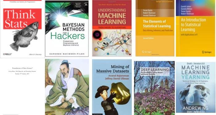
Here is a quick collection of such books to start your fair weather study off on the right foot. The list begins with a base of statistics, moves on to machine learning foundations, progresses to a few bigger picture titles, has a quick look at an advanced topic or 2, and ends off with something that brings it all together. A mix of classic and contemporary titles, hopefully you find something new (to you) and of interest here.
Think Stats is an introduction to Probability and Statistics for Python programmers.
Think Stats emphasizes simple techniques you can use to explore real data sets and answer interesting questions. The book presents a case study using data from the National Institutes of Health. Readers are encouraged to work on a project with real datasets.
An intro to Bayesian methods and probabilistic programming from a computation/understanding-first, mathematics-second point of view.
The Bayesian method is the natural approach to inference, yet it is hidden from readers behind chapters of slow, mathematical analysis. The typical text on Bayesian inference involves two to three chapters on probability theory, then enters what Bayesian inference is. Unfortunately, due to mathematical intractability of most Bayesian models, the reader is only shown simple, artificial examples. This can leave the user with a so-what feeling about Bayesian inference. In fact, this was the author's own prior opinion.
Machine learning is one of the fastest growing areas of computer science, with far-reaching applications. The aim of this textbook is to introduce machine learning, and the algorithmic paradigms it offers, in a principled way. The book provides a theoretical account of the fundamentals underlying machine learning and the mathematical derivations that transform these principles into practical algorithms. Following a presentation of the basics, the book covers a wide array of central topics unaddressed by previous textbooks. These include a discussion of the computational complexity of learning and the concepts of convexity and stability; important algorithmic paradigms including stochastic gradient descent, neural networks, and structured output learning; and emerging theoretical concepts such as the PAC-Bayes approach and compression-based bounds.
This book descibes the important ideas in these areas in a common conceptual framework. While the approach is statistical, the emphasis is on concepts rather than mathematics. Many examples are given, with a liberal use of color graphics. It should be a valuable resource for statisticians and anyone interested in data mining in science or industry. The book's coverage is broad, from supervised learning (prediction) to unsupervised learning. The many topics include neural networks, support vector machines, classification trees and boosting--the first comprehensive treatment of this topic in any book.
This book provides an introduction to statistical learning methods. It is aimed for upper level undergraduate students, masters students and Ph.D. students in the non-mathematical sciences. The book also contains a number of R labs with detailed explanations on how to implement the various methods in real life settings, and should be a valuable resource for a practicing data scientist.
While traditional areas of computer science remain highly important, increasingly researchers of the future will be involved with using computers to understand and extract usable information from massive data arising in applications, not just how to make computers useful on specific well-defined problems. With this in mind we have written this book to cover the theory likely to be useful in the next 40 years, just as an understanding of automata theory, algorithms, and related topics gave students an advantage in the last 40 years.
This guide follows a learn-by-doing approach. Instead of passively reading the book, I encourage you to work through the exercises and experiment with the Python code I provide. I hope you will be actively involved in trying out and programming data mining techniques. The textbook is laid out as a series of small steps that build on each other until, by the time you complete the book, you have laid the foundation for understanding data mining techniques.
The book is based on Stanford Computer Science course CS246: Mining Massive Datasets (and CS345A: Data Mining).
The book, like the course, is designed at the undergraduate computer science level with no formal prerequisites. To support deeper explorations, most of the chapters are supplemented with further reading references.
9. Deep Learning By Ian Goodfellow, Yoshua Bengio and Aaron Courville
The Deep Learning textbook is a resource intended to help students and practitioners enter the field of machine learning in general and deep learning in particular. The online version of the book is now complete and will remain available online for free.
AI, Machine Learning and Deep Learning are transforming numerous industries. But building a machine learning system requires that you make practical decisions:
Should you collect more training data?
Should you use end-to-end deep learning?
How do you deal with your training set not matching your test set?
and many more.
Historically, the only way to learn how to make these "strategy" decisions has been a multi-year apprenticeship in a graduate program or company. I am writing a book to help you quickly gain this skill, so that you can become better at building AI systems.
Google’s TensorFlow has been a hot topic in deep learning recently. The open source software, designed to allow efficient computation of data flow graphs, is especially suited to deep learning tasks. It is designed to be executed on single or multiple CPUs and GPUs, making it a good option for complex deep learning tasks. In it’s most recent incarnation – version 1.0 – it can even be run on certain mobile operating systems.
This introductory tutorial to TensorFlow will give an overview of some of the basic concepts of TensorFlow in Python. These will be a good stepping stone to building more complex deep learning networks, such as Convolution Neural Networks and Recurrent Neural Networks, in the package. We’ll be creating a simple three-layer neural network to classify the MNIST dataset. This tutorial assumes that you are familiar with the basics of neural networks, which you can get up to scratch with in the neural networks tutorial if required. To install TensorFlow, follow the instructions here. First, let’s have a look at the main ideas of TensorFlow.
1.0 TensorFlow graphs
TensorFlow is based on graph based computation – “what on earth is that?”, you might say. It’s an alternative way of conceptualising mathematical calculations. Consider the following expression a=(b+c)∗(c+2) . We can break this function down into the following components:
dea=b+c=c+2=d∗c
Now we can represent these operations graphically as:
Simple computational graph
This may seem like a silly example – but notice a powerful idea in expressing the equation this way: two of the computations (d=b+c and e=c+2 ) can be performed in parallel. By splitting up these calculations across CPUs or GPUs, this can give us significant gains in computational times. These gains are a must for big data applications and deep learning – especially for complicated neural network architectures such as Convolutional Neural Networks (CNNs) and Recurrent Neural Networks (RNNs). The idea behind TensorFlow is to ability to create these computational graphs in code and allow significant performance improvements via parallel operations and other efficiency gains.
We can look at a similar graph in TensorFlow below, which shows the computational graph of a three-layer neural network.
TensorFlow data flow graph
The animated data flows between different nodes in the graph are tensors which are multi-dimensional data arrays. For instance, the input data tensor may be 5000 x 64 x 1, which represents a 64 node input layer with 5000 training samples. After the input layer there is a hidden layer with rectified linear units as the activation function. There is a final output layer (called a “logit layer” in the above graph) which uses cross entropy as a cost/loss function. At each point we see the relevant tensors flowing to the “Gradients” block which finally flow to the Stochastic Gradient Descent optimiser which performs the back-propagation and gradient descent.
Here we can see how computational graphs can be used to represent the calculations in neural networks, and this, of course, is what TensorFlow excels at. Let’s see how to perform some basic mathematical operations in TensorFlow to get a feel for how it all works.
2.0 A Simple TensorFlow example
Let’s first make TensorFlow perform our little example calculation above – a=(b+c)∗(c+2) . First we need to introduce ourselves to TensorFlow variables and constants. Let’s declare some then I’ll explain the syntax:
import tensorflow as tf
# first, create a TensorFlow constantconst= tf.constant(2.0, name="const")# create TensorFlow variables
b = tf.Variable(2.0, name='b')
c = tf.Variable(1.0, name='c')
As can be observed above, TensorFlow constants can be declared using the tf.constant function, and variables with the tf.Variable function. The first element in both is the value to be assigned the constant / variable when it is initialised. The second is an optional name string which can be used to label the constant / variable – this is handy for when you want to do visualisations (as will be discussed briefly later). TensorFlow will infer the type of the constant / variable from the initialised value, but it can also be set explicitly using the optional dtype argument. TensorFlow has many of its own types like tf.float32, tf.int32 etc. – see them all here.
It’s important to note that, as the Python code runs through these commands, the variables haven’t actually been declared as they would have been if you just had a standard Python declaration (i.e. b = 2.0). Instead, all the constants, variables, operations and the computational graph are only created when the initialisation commands are run.
Next, we create the TensorFlow operations:
# now create some operations
d = tf.add(b, c, name='d')
e = tf.add(c,const, name='e')
a = tf.multiply(d, e, name='a')
TensorFlow has a wealth of operations available to perform all sorts of interactions between variables, some of which we’ll get to later in the tutorial. The operations above are pretty obvious, and they instantiate the operations b+c , c+2.0 and d∗e .
The next step is to setup an object to initialise the variables and the graph structure:
# setup the variable initialisation
init_op = tf.global_variables_initializer()
Ok, so now we are all set to go. To run the operations between the variables, we need to start a TensorFlow session – tf.Session. The TensorFlow session is an object where all operations are run. Using the with Python syntax, we can run the graph with the following code:
# start the sessionwith tf.Session()as sess:# initialise the variables
sess.run(init_op)# compute the output of the graph
a_out = sess.run(a)print("Variable a is {}".format(a_out))
The first command within the with block is the initialisation, which is run with the, well, run command. Next we want to figure out what the variable a should be. All we have to do is run the operation which calculates a i.e. a = tf.multiply(d, e, name=’a’). Note that a is an operation, not a variable and therefore it can be run. We do just that with the sess.run(a) command and assign the output to a_out, the value of which we then print out.
Note something cool – we defined operations d and e which need to be calculated before we can figure out what a is. However, we don’t have to explicitly run those operations, as TensorFlow knows what other operations and variables the operation a depends on, and therefore runs the necessary operations on its own. It does this through its data flow graph which shows it all the required dependencies. Using the TensorBoard functionality, we can see the graph that TensorFlow created in this little program:
Simple TensorFlow graph
Now that’s obviously a trivial example – what if we had an array of b values that we wanted to calculate the value of a over?
2.1 The TensorFlow placeholder
Let’s also say that we didn’t know what the value of the array b would be during the declaration phase of the TensorFlow problem (i.e. before the with tf.Session() as sess) stage. In this case, TensorFlow requires us to declare the basic structure of the data by using the tf.placeholder variable declaration. Let’s use it for b:
# create TensorFlow variables
b = tf.placeholder(tf.float32,[None,1], name='b')
Because we aren’t providing an initialisation in this declaration, we need to tell TensorFlow what data type each element within the tensor is going to be. In this case, we want to use tf.float32. The second argument is the shape of the data that will be “injected” into this variable. In this case, we want to use a (? x 1) sized array – because we are being cagey about how much data we are supplying to this variable (hence the “?”), the placeholder is willing to accept a None argument in the size declaration. Now we can inject as much 1-dimensional data that we want into the b variable.
The only other change we need to make to our program is in the sess.run(a,…) command:
Note that we have added the feed_dict argument to the sess.run(a,…) command. Here we remove the mystery and specify exactly what the variable b is to be – a one-dimensional range from 0 to 10. As suggested by the argument name, feed_dict, the input to be supplied is a Python dictionary, with each key being the name of the placeholder that we are filling.
When we run the program again this time we get:
Variable a is[[3.][6.][9.][12.][15.][18.][21.][24.][27.][30.]]
Notice how TensorFlow adapts naturally from a scalar output (i.e. a singular output when a=9.0) to a tensor (i.e. an array/matrix)? This is based on its understanding of how the data will flow through the graph.
Now we are ready to build a basic MNIST predicting neural network.
3.0 A Neural Network Example
Now we’ll go through an example in TensorFlow of creating a simple three layer neural network. In future articles, we’ll show how to build more complicated neural network structures such as convolution neural networks and recurrent neural networks. For this example though, we’ll keep it simple. If you need to scrub up on your neural network basics, check out my popular tutorial on the subject. In this example, we’ll be using the MNIST dataset (and its associated loader) that the TensorFlow package provides. This MNIST dataset is a set of 28×28 pixel grayscale images which represent hand-written digits. It has 55,000 training rows, 10,000 testing rows and 5,000 validation rows.
We can load the data by running:
from tensorflow.examples.tutorials.mnist import input_data
mnist = input_data.read_data_sets("MNIST_data/", one_hot=True)
The one_hot=True argument specifies that instead of the labels associated with each image being the digit itself i.e. “4”, it is a vector with “one hot” node and all the other nodes being zero i.e. [0, 0, 0, 0, 1, 0, 0, 0, 0, 0]. This lets us easily feed it into the output layer of our neural network.
3.1 Setting things up
Next, we can set-up the placeholder variables for the training data (and some training parameters):
# Python optimisation variables
learning_rate =0.5
epochs =10
batch_size =100# declare the training data placeholders# input x - for 28 x 28 pixels = 784
x = tf.placeholder(tf.float32,[None,784])# now declare the output data placeholder - 10 digits
y = tf.placeholder(tf.float32,[None,10])
Notice the x input layer is 784 nodes corresponding to the 28 x 28 (=784) pixels, and the y output layer is 10 nodes corresponding to the 10 possible digits. Again, the size of x is (? x 784), where the ? stands for an as yet unspecified number of samples to be input – this is the function of the placeholder variable.
Now we need to setup the weight and bias variables for the three layer neural network. There are always L-1 number of weights/bias tensors, where L is the number of layers. So in this case, we need to setup two tensors for each:
# now declare the weights connecting the input to the hidden layer
W1 = tf.Variable(tf.random_normal([784,300], stddev=0.03), name='W1')
b1 = tf.Variable(tf.random_normal([300]), name='b1')# and the weights connecting the hidden layer to the output layer
W2 = tf.Variable(tf.random_normal([300,10], stddev=0.03), name='W2')
b2 = tf.Variable(tf.random_normal([10]), name='b2')
Ok, so let’s unpack the above code a little. First, we declare some variables for W1 and b1, the weights and bias for the connections between the input and hidden layer. This neural network will have 300 nodes in the hidden layer, so the size of the weight tensor W1 is [784, 300]. We initialise the values of the weights using a random normal distribution with a mean of zero and a standard deviation of 0.03. TensorFlow has a replicated version of the numpy random normal function, which allows you to create a matrix of a given size populated with random samples drawn from a given distribution. Likewise, we create W2 and b2 variables to connect the hidden layer to the output layer of the neural network.
Next, we have to setup node inputs and activation functions of the hidden layer nodes:
# calculate the output of the hidden layer
hidden_out = tf.add(tf.matmul(x, W1), b1)
hidden_out = tf.nn.relu(hidden_out)
In the first line, we execute the standard matrix multiplication of the weights (W1) by the input vector x and we add the bias b1. The matrix multiplication is executed using the tf.matmul operation. Next, we finalise the hidden_out operation by applying a rectified linear unit activation function to the matrix multiplication plus bias. Note that TensorFlow has a rectified linear unit activation already setup for us, tf.nn.relu.
# now calculate the hidden layer output - in this case, let's use a softmax activated# output layer
y_ = tf.nn.softmax(tf.add(tf.matmul(hidden_out, W2), b2))
Again we perform the weight multiplication with the output from the hidden layer (hidden_out) and add the bias, b2. In this case, we are going to use a softmax activation for the output layer – we can use the included TensorFlow softmax function tf.nn.softmax.
We also have to include a cost or loss function for the optimisation / backpropagation to work on. Here we’ll use the cross entropy cost function, represented by:
Where y(i)j is the ith training label for output node j, yj_(i) is the ith predicted label for output node j, m is the number of training / batch samples and n is the number . There are two operations occurring in the above equation. The first is the summation of the logarithmic products and additions across all the output nodes. The second is taking a mean of this summation across all the training samples. We can implement this cross entropy cost function in TensorFlow with the following code:
Some explanation is required. The first line is an operation converting the output y_ to a clipped version, limited between 1e-10 to 0.999999. This is to make sure that we never get a case were we havea log(0) operation occurring during training – this would return NaN and break the training process. The second line is the cross entropy calculation.
To perform this calculation, first we use TensorFlow’s tf.reduce_sum function – this function basically takes the sum of a given axis of the tensor you supply. In this case, the tensor that is supplied is the element-wise cross-entropy calculation for a single node and training sample i.e.: y(i)jlog(yj_(i))+(1–y(i)j)log(1–yj_(i)) . Remember that y and y_clipped in the above calculation are (m x 10) tensors – therefore we need to perform the first sum over the second axis. This is specified using the axis=1 argument, where “1” actually refers to the second axis when we have a zero-based indices system like Python.
After this operation, we have an (m x 1) tensor. To take the mean of this tensor and complete our cross entropy cost calculation (i.e. execute this part 1m∑mi=1 ), we use TensorFlow’s tf.reduce_mean function. This function simply takes the mean of whatever tensor you provide it. So now we have a cost function that we can use in the training process.
Let’s setup the optimiser in TensorFlow:
# add an optimiser
optimiser = tf.train.GradientDescentOptimizer(learning_rate=learning_rate).minimize(cross_entropy)
Here we are just using the gradient descent optimiser provided by TensorFlow. We initialize it with a learning rate, then specify what we want it to do – i.e. minimise the cross entropy cost operation we created. This function will then perform the gradient descent (for more details on gradient descent see here and here) and the backpropagation for you. How easy is that? TensorFlow has a library of popular neural network training optimisers, see here.
Finally, before we move on to the main show, were we actually run the operations, let’s setup the variable initialisation operation and an operation to measure the accuracy of our predictions:
The correct prediction operation correct_prediction makes use of the TensorFlow tf.equal function which returns True or False depending on whether to arguments supplied to it are equal. The tf.argmax function is the same as the numpy argmax function, which returns the index of the maximum value in a vector / tensor. Therefore, the correct_prediction operation returns a tensor of size (m x 1) of True and False values designating whether the neural network has correctly predicted the digit. We then want to calculate the mean accuracy from this tensor – first we have to cast the type of the correct_prediction operation from a Boolean to a TensorFlow float in order to perform the reduce_mean operation. Once we’ve done that, we now have an accuracy operation ready to assess the performance of our neural network.
3.2 Setting up the training
We now have everything we need to setup the training process of our neural network. I’m going to show the full code below, then talk through it:
# start the sessionwith tf.Session()as sess:# initialise the variables
sess.run(init_op)
total_batch =int(len(mnist.train.labels)/ batch_size)for epoch in range(epochs):
avg_cost =0for i in range(total_batch):
batch_x, batch_y = mnist.train.next_batch(batch_size=batch_size)
_, c = sess.run([optimiser, cross_entropy],
feed_dict={x: batch_x, y: batch_y})
avg_cost += c / total_batch
print("Epoch:",(epoch +1),"cost =","{:.3f}".format(avg_cost))print(sess.run(accuracy, feed_dict={x: mnist.test.images, y: mnist.test.labels}))
Stepping through the lines above, the first couple relate to setting up the with statement and running the initialisation operation. The third line relates to our mini-batch training scheme that we are going to run for this neural network. If you want to know about mini-batch gradient descent, check out this post. In the third line, we are calculating the number of batches to run through in each training epoch. After that, we loop through each training epoch and initialise an avg_cost variable to keep track of the average cross entropy cost for each epoch. The next line is where we extract a randomised batch of samples, batch_x and batch_y, from the MNIST training dataset. The TensorFlow provided MNIST dataset has a handy utility function, next_batch, that makes it easy to extract batches of data for training.
The following line is where we run two operations. Notice that sess.run is capable of taking a list of operations to run as its first argument. In this case, supplying [optimiser, cross_entropy] as the list means that both these operations will be performed. As such, we get two outputs, which we have assigned to the variables _ and c. We don’t really care too much about the output from the optimiser operation but we want to know the output from the cross_entropy operation – which we have assigned to the variable c. Note, we run the optimiser (and cross_entropy) operation on the batch samples. In the following line, we use c to calculate the average cost for the epoch.
Finally, we print out our progress in the average cost, and after the training is complete, we run the accuracy operation to print out the accuracy of our trained network on the test set. Running this program produces the following output:
There we go – approximately 98% accuracy on the test set, not bad. We could do a number of things to improve the model, such as regularisation (see this tips and tricks post), but here we are just interested in exploring TensorFlow. You can also use TensorBoard visualisation to look at things like the increase in accuracy over the epochs:
TensorBoard plot of the increase in accuracy over 10 epochs
In a future article, I’ll introduce you to TensorBoard visualisation, which is a really nice feature of TensorFlow. For now, I hope this tutorial was instructive and helps get you going on the TensorFlow journey – in future articles I’ll show you how to build more complex neural networks such as convolution neural networks and recurrent neural networks. So stay tuned.
GitHub - duggalrahul/AlexNet-Experiments-Keras: Code examples for training AlexNet using Keras and Theano https://github.com/duggalrahul/AlexNet-Experiments-Keras
As a lot of you read, Baidu has released their paper on speech-to-text called DeepSpeech. As written in paper, their end-to-end architecture offers 7x speed-up over previous architectures. And as I understand - sets the new state-of-the-art.
Papers are fun, but without data and code their hard to implement for a lot of individuals.
Great thing is that mozilla open-sourced DeepSpeech model that is implemented in Tensorflow. So now all of us can use it, tweak it, train it.
We often think of Momentum as a means of dampening oscillations and speeding up the iterations, leading to faster convergence. But it has other interesting behavior. It allows a larger range of step-sizes to be used, and creates its own oscillations. What is going on?
Here’s a popular story about momentum [1, 2, 3]: gradient descent is a man walking down a hill. He follows the steepest path downwards, his progress is slow, but steady. Momentum is a heavy ball rolling down the same hill. The added inertia acts both as a smoother and an accelerator, dampening oscillations and causing us to barrel through narrow valleys, small humps and local minima.
This standard story isn’t wrong, but it fails to explain many important behaviors of momentum. In fact, momentum can be understood far more precisely if we study it on the right model.
One nice model is the convex quadratic. This model is rich enough to reproduce momentum’s local dynamics in real problems, and yet simple enough to be understood in closed form. This balance gives us powerful traction for understanding this algorithm.
We begin with Gradient Descent. The algorithm has as many virtues, but speed is not one of them. It is simple -- when optimizing a smooth function f, we make a small step in the gradient wk+1=wk−α∇f(wk). For a step size small enough, gradient descent makes a monotonic improvement at every iteration. It always converges, albeit to a local minimum. And under a few weak curvature conditions it can even get there at an exponential rate.
But the exponential decrease, though appealing in theory, can often be infuriatingly small. Things often begin quite well -- with an impressive, almost immediate decrease in the loss. But as the iterations progress, things start to slow down. You start to get a nagging feeling you're not making as much progress as you should be. What has gone wrong?
The problem could be the optimizer's old nemesis, pathological curvature. Pathological curvature is, simply put, regions of f which aren't scaled properly. The landscapes are often described as a valleys, trenches, canals and ravines. The iterates either jump between valleys, or approach the optimum in small, timid steps. Progress along certain directions grind to a halt. In these unfortunate regions, gradient descent fumbles.
Momentum proposes the following tweak to gradient descent. We give gradient descent a short-term memory: zk+1wk+1=βzk+∇f(wk)=wk−αzk+1 the change is innocent, and costs almost nothing. When β=0 , we recover gradient descent. But for β=0.99 (sometimes 0.999, if things are really bad), this appears to be the boost we need. Our iterations regain that speed and boldness it lost, speeding to the optimum with a renewed energy.
Optimizers call this minor miracle "acceleration".
The new algorithm may seem at first glance like a cheap hack. A simple trick to get around gradient descent's more aberrant behavior - a smoother for oscillations between steep canyons. But the truth, if anything, is the other way round. It is gradient descent which is the hack. First, momentum gives up to a quadratic speedup on many functions. 1 This is no small matter -- this is similar to the speedup you get from the Fast Fourier Transform, Quicksort, and Grover's Algorithm. When the universe gives you quadratic speedups, you should start to pay attention.
But there's more. A lower bound, courtesy of Nesterov [5], states that momentum is, in a certain very narrow and technical sense, optimal. Now, this doesn't mean it is the best algorithm for all functions in all circumstances. But it does satisfy some curiously beautiful mathematical properties which scratch a very human itch for perfection and closure. But more on that later. Let's say this for now -- momentum is an algorithm for the book.
First Steps: Gradient Descent
We begin by studying gradient descent on the simplest model possible which isn't trivial -- the convex quadratic, f(w)=21wTAw−bTw,w∈Rn. When A is invertible, the optimal solution w⋆ occurs at w⋆=A−1b. Simple as this model may be, it is rich enough to approximate many functions (think of A as your favorite model of curvature -- the Hessian, Fisher Information Matrix [6], etc) and captures all the key features of pathological curvature. And more importantly, we can write an exact closed formula for gradient descent on this function.
This is how it goes. Since ∇f(w)=Aw−b, the iterates are wk+1=wk−α(Awk−b) Here's the trick. There is a very natural space to view gradient descent where all the dimensions act independently - the eigenvectors of A.
Every symmetric matrix A has an eigenvalue decomposition A=Qdiag(λ1,…,λn)QT,Q=[q1,…,qn], and as per convention, we will assume that the λi's are sorted, from smallest λ1 to biggest λn. If we perform a change of basis, xk=QT(wk−w⋆), the iterations break apart, becoming: xik+1=xik−αλixik=(1−αλi)xik=(1−αλi)kxi0 Moving back to our original space w, we can see that wk−w⋆=Qxk=i∑nxi0(1−αλi)kqi and there we have it - gradient descent in closed form.
Decomposing the Error
The above equation admits a simple interpretation. Each element of x0 is the component of the error in the initial guess in Q-basis. There are n such errors, and each of these errors follow their own, solitary path to the minimum, decreasing exponentially with a compounding rate of 1−αλi. The closer that number is to 1, the slower it converges.
For most step-sizes, the eigenvectors with largest eigenvalues converge the fastest. This triggers an explosion of progress in the first few iterations, before things slow down as the smaller eigenvector's struggles are revealed. By writing the contributions of each eigenspaces's error to the loss f(wk)−f(w⋆)=∑(1−αλi)2kλi[xi0]2 we can visualize the contributions of each error component to the loss.
Optimization can be seen as combination of several component problems, shown here as 1 2 3 with eigenvalues λ1=0.01, λ2=0.1, and λ3=1 respectively.
Step Size
Optimal Step Size
Choosing A Step-size
The above analysis gives us immediate guidance as to how to set a step-size α. In order to converge, each ∣1−αλi∣ must be strictly less than 1. All workable step-sizes, therefore, fall in the interval 0<αλi<2. The overall convergence rate is determined by the slowest error component, which must be either λ1 or λn: rate(α)=imax∣1−αλi∣=max{∣1−αλ1∣,∣1−αλn∣}
This overall rate is minimized when the rates for λ1 and λn are the same -- this mirrors our informal observation in the previous section that the optimal step size causes the first and last eigenvectors to converge at the same time. If we work this through we get: optimal α=αargminrate(α)optimal rate=αminrate(α)=λ1+λn2=λn/λ1+1λn/λ1−1
Notice the ratio λn/λ1 determines the convergence rate of the problem. In fact, this ratio appears often enough that we give it a name, and a symbol - the condition number. condition number:=κ:=λ1λn The condition number means many things. It is a measure of how close to singular a matrix is. It is a measure of how robust A−1b is to perturbations in b. And in this context, the condition number gives us a measure of how poorly gradient descent will perform. A ratio of κ=1 is ideal, giving convergence in one step (of course, the function is trivial). Unfortunately the larger the ratio, the slower gradient descent will be. The condition number is therefore a direct measure pathological of curvature.
Example: Polynomial Regression
The above analysis reveals an insight : all errors are not made equal. Indeed, there are different kinds of errors, n to be exact, one for each of the eigenvectors of A. And gradient descent is better at correcting some kinds of errors than others. But what do the eigenvectors of A mean? Surprisingly, in many applications they admit a very concrete interpretation.
Lets see how this plays out in polynomial regression. Given 1D data, ξi, our problem is to fit the model model(ξ)=w1p1(ξ)+⋯+wnpn(ξ)pi=ξ↦ξi−1 to our observations, di. This model, though nonlinear in the input ξ is linear in the weights, and therefore we can write the model as a linear combination of monomials, like:
Because of the linearity, we can fit this model at our data ξi using linear regression on the model mismatch minimizew21i∑(model(ξi)−di)2=21∥Zw−d∥2 where Z=⎝⎜⎜⎛11⋮1ξ1ξ2⋮ξmξ12ξ22⋮ξm2……⋱…ξ1n−1ξ2n−1⋮ξmn−1⎠⎟⎟⎞.
The path of convergence, as we know, is elucidated when we view the iterates in the space of Q (the eigenvectors of ZTZ). So let's recast our regression problem in the basis of Q. First, we do a change of basis, by rotating w into Qw, and counter-rotating our feature maps p into eigenspace, p¯. We can now conceptualize the same regression as one over a different polynomial basis, with the model model(ξ)=x1p¯1(ξ)+⋯+xnp¯n(ξ)p¯i=∑qijpj. This model is identical to the old one. But these new features p¯ (which I call "eigenfeatures") and weights have the pleasing property that each coordinate acts independently of the others. Now our optimization problem breaks down, really, into n small 1D optimization problems. And each coordinate can be optimized greedily and independently, one at a time in any order, to produce the final, global, optimum. The eigenfeatures are also much more informative,
The observations in the above diagram can be justified mathematically. From a statistical point of view, we would like a model which is in some sense, robust to noise. Our model cannot possibly be meaningful if the slightest perturbation to the observations changes the entire model dramatically. And the eigenfeatures, the principle components of the data, give us exactly the decomposition we need to sort the features by its sensitivity to perturbations in di's. The most robust components appear in the front (with the largest eigenvalues), and the most sensitive components in the back (with the smallest eigenvalues).
This measure of robustness, by a rather convenient coincidence, is also a measure of how easily an eigenspace converges. And thus, the "pathological directions" -- the eigenspaces which converge the slowest -- are also those which are most sensitive to noise! So starting at a simple initial point like 0 (by a gross abuse of language, let's think of this as a prior), we track the iterates till a desired level of complexity is reached. Let's see how this plays out in gradient descent.
This effect is harnessed with the heuristic of early stopping : by stopping the optimization early, you can often get better generalizing results. Indeed, the effect of early stopping is very similar to that of more conventional methods of regularization, such as Tikhonov Regression. Both methods try to suppress the components of the smallest eigenvalues directly, though they employ different methods of spectral decay.2 But early stopping has a distinct advantage. Once the stepsize is chosen, there are no regularization parameters to fiddle with. Indeed, in the course of a single optimization, we have the entire family of models, from underfitted to overfitted, at our disposal. This gift, it seems, doesn't to come at a price. A beautiful free lunch [7] indeed.
The Dynamics of Momentum
Let's turn our attention back to momentum. Recall the momentum update is zk+1wk+1=βzk+∇f(wk)=wk−αzk+1. Since ∇f(wk)=Awk−b, the update on the quadratic is zk+1wk+1=βzk+(Awk−b)=wk−αzk+1 following [8], we go through the same motions, with the change of basis xk=Q(wk−w⋆) and yk=Qzk to yield the update rule yik+1xik+1=βyik+λixik=xik−αyik+1. in which each component of acts independently of the other components (though xik and yik are coupled). This lets us rewrite our iterates as 3(yikxik)=Rk(yi0xi0)R=(β−αβλi1−αλi). There are many ways of taking a matrix to the kth power. But for the 2×2 case there is an elegant and little known formula [9] in terms of the eigenvectors of R, σ1 and σ2. Rk={σ1kR1−σ2kR2σ1k(kR/σ1−(k−1)I)σ1≠σ2σ1=σ2,Rj=σ1−σ2R−σjI This formula is rather complicated, but the takeaway here is that it plays the exact same role the individual convergence rates, 1−αλi do in gradient descent. But instead of one geometric series, we have two coupled series, which may have real or complex values. The convergence rate is therefore the slowest of the two rates, max{∣σ1∣,∣σ2∣}4. By plotting this out, we see there are distinct regions of the parameter space which reveal a rich taxonomy of convergence behavior [10]:
Convergence Rate
A plot of max{∣σ1∣,∣σ2∣} reveals distinct regions, each with its own style of convergence.
For what values of α and β does momentum converge? Since we need both σ1 and σ2 to converge, our convergence criteria is now max{∣σ1∣,∣σ2∣}<1. The range of available step-sizes work out 5 to be 0<αλi<2+2βfor0≤β<1 We recover the previous result for gradient descent when β=0. But notice an immediate boon we get. Momentum allows us to a crank up the step-size up by a factor of 2 before diverging.
The Critical Damping Coefficient
The true magic happens, however, when we find the sweet spot of α and β. Let us try to first optimize over β.
Momentum admits an interesting physical interpretation when α is [11] small: it is a discretization of a damped harmonic oscillator. Consider a physical simulation operating in discrete time (like a video game).
yik+1=+λixikand perturbed by an external force field We can think of −yik as velocityβyikwhich is dampened at each step xik+1=xik−αyik+1And x is our particle's positionwhich is moved at each step by a small amount in the direction of the velocity yik+1.
We can break this equation apart to see how each component affects the dynamics of the system. Here we plot, for 150 iterates, the particle's velocity (the horizontal axis) against its position (the vertical axis), in a phase diagram.
This system is best imagined as a weight suspended on a spring. We pull the weight down by one unit, and we study the path it goes as it returns to equilibrium. In the analogy, the spring is the source of our external force λixik, and equilibrium is the state when both the position xik, and the speed, yik are 0. The choice of β crucially affects the rate of return to equilibrium.
The critical β=(1−√αλi)2 gives us a convergence rate (in eigenspace i) of 1−√αλi. A square root improvement over gradient descent, 1−αλi! Alas, this only applies to the error in the ith eigenspace, with α fixed.
Optimal parameters
To get a global convergence rate, we must optimize over both α and β. This is a more complicated affair,6 but they work out to be α=(√λ1+√λn2)2β=(√λn+√λ1√λn−√λ1)2 Plug this into the convergence rate, and you get
With barely a modicum of extra effort, we have essentially square rooted the condition number! These gains, in principle, require explicit knowledge of λ1 and λn. But the formulas reveal a simple guideline. When the problem's conditioning is poor, the optimal α is approximately twice that of gradient descent, and the momentum term is close to 1. So set β as close to 1 as you can, and then find the highest α which still converges. Being at the knife's edge of divergence, like in gradient descent, is a good place to be.
We can do the same decomposition here with momentum, with eigenvalues λ1=0.01, λ2=0.1, and λ3=1. Though the decrease is no longer monotonic, but significantly faster. f(wk)−f(w⋆) Note that the optimal parameters do not necessarily imply the fastest convergence, though, only the fastest asymptotic convergence rate.
Step size α =
Momentum β =
While the loss function of gradient descent had a graceful, monotonic curve, optimization with momentum displays clear oscillations. These ripples are not restricted to quadratics, and occur in all kinds of functions in practice. They are not cause for alarm, but are an indication that extra tuning of the hyperparameters is required.
Example: The Colorization Problem
Lets look at how momentum accelerates convergence with a concrete example. On a grid of pixels let G be the graph with vertices as pixels, E be the set of edges connecting each pixel to its four neighboring pixels, and D be a small set of a few distinguished vertices. Consider the problem of minimizing
minimize21i∈D∑(wi−1)2The colorizer pulls distinguished pixels towards 1 +21i,j∈E∑(wi−wj)2.The smoother spreads out the color
The optimal solution to this problem is a vector of all 1's 7. An inspection of the gradient iteration reveals why we take a long time to get there. The gradient step, for each component, is some form of weighted average of the current value and its neighbors: wik+1=wik−αj∈N∑(wik−wjk)−{α(wik−1)0i∈Di∉D This kind of local averaging is effective at smoothing out local variations in the pixels, but poor at taking advantage of global structure. The updates are akin to a drop of ink, diffusing through water. Movement towards equilibrium is made only through local corrections and so left undisturbed, its march towards the solution is slow and laborious. Fortunately, momentum speeds things up significantly.
The eigenvectors of the colorization problem form a generalized Fourier basis for Rn. The smallest eigenvalues have low frequencies, hence gradient descent corrects high frequency errors well but not low frequency ones.
In vectorized form, the colorization problem is
minimizeThe smoother's quadratic form is the Graph Laplacian21i∈D∑(xTeieiTx−eiTx)+21xTLGxAnd the colorizer is a small low rank correction with a linear term. ei is the ith unit vector.
The Laplacian matrix ,LG8, which dominates the behavior of the optimization problem, is a valuable bridge between linear algebra and graph theory. This is a rich field of study, but one fact is pertinent to our discussion here. The conditioning of LG, here defined as the ratio of the second eigenvector to the last (the first eigenvalue is always 0, with eigenvector equal to the matrix of all 1's), is directly connected to the connectivity of the graph.
Small world graphs, like expanders and dense graphs, have excellent conditioningThe conditioning of grids improves with its dimensionality.And long, wiry graphs, like paths, condition poorly.
This observations carries through to the colorization problem, and the intuition behind this should be clear. Well connected graphs allow rapid diffusion of information through the edges, while graphs with poor connectivity do not. And this principle, taken to the extreme, furnishes a class of functions so hard to optimize they reveal the limits of first order optimization.
The Limits of Descent
Let's take a step back. We have, with a clever trick, improved the convergence of gradient descent by a quadratic factor with the introduction of a single auxiliary sequence. But is this the best we can do? Could we improve convergence even more with two sequences? Could one perhaps choose the α's and β's intelligently and adaptively? It is tempting to ride this wave of optimism - to the cube root and beyond!
Unfortunately, while improvements to the momentum algorithm do exist, they all run into a certain, critical, almost inescapable lower bound.
Adventures in Algorithmic Space
To understand the limits of what we can do, we must first formally define the algorithmic space in which we are searching. Here's one possible definition. The observation we will make is that both Gradient Descent and momentum can be "unrolled". Indeed, since w1w2wk===⋮=w0−α∇f(w0)w1−α∇f(w1)w0−α∇f(w0)−α∇f(w1)w0−α∇f(w0)−⋯⋯−α∇f(wk) we can write gradient descent as: wk=w0−αi∑k∇f(wi) A similar trick can be done with momentum, wk=w0+αi∑k1−β(1−βi)∇f(wi) In fact, all manner of first order algorithms, including the Conjugate Gradient algorithm, AdaMax, Averaged Gradient and more can be written in (though not quite so neatly) this unrolled form. Therefore the class of algorithms for which wk=w0+i∑kγik∇f(wi) for some γik contains momentum, gradient descent and a whole bunch of other algorithms you might dream up. This is what is assumed in Assumption 2.1.4 [5] of Nesterov. But let's push this even further, and expand this class to allow different step sizes for different directions. wk=w0+i∑kΓik∇f(wi) for some diagonal matrix Γik. This class of methods covers most of the popular algorithms for training neural networks, including ADAM and AdaGrad. We shall refer to this class of methods as "Linear First Order Methods", and we will show a single function all these methods ultimately fail on.
The Resisting Oracle
Earlier, when we talked about the colorizer problem, we observed that wiry graphs cause bad conditioning in our optimization problem. Taking this to its extreme, we can look at a graph consisting of a single path -- a function so badly conditioned that Nesterov called a variant of it "the worst function in the world". The function follows the same structure as the colorizer problem, and we shall call this the Convex Rosenbrock,
fn(w)=with a colorizer of one node 21(w1−1)2+21i=1∑n(wi−wi+1)2strong couplings adjacent nodes in the path, +κ−12∥w∥2and a small regularization term.
The optimal solution of this problem is wi⋆=(√κ+1√κ−1)i and the condition number of the problem fn approaches κ as n goes to infinity. Now observe the behavior of the momentum algorithm on this function, starting from w0=0.
Step size α =
Momentum β =
Here we see the first 50 iterates of momentum on the Convex Rosenbrock for n=25. The behavior here is similar to that of any Linear First Order Algorithm.
This triangle is a "dead zone" of our iterates. The iterates are always 0, no matter what the parameters. The remaining expanding space is the "light cone" of our iterate's influence. Momentum does very well here with the optimal parameters.
Error
Weights
The observations made in the above diagram are true for any Linear First Order algorithm. Let us prove this. First observe that each component of the gradient depends only on the values directly before and after it: ∇f(x)i=2wi−wi−1−wi+1+κ−14wi,i≠1. Therefore the fact we start at 0 guarantees that that component must remain stoically there till an element either before and after it turns nonzero. And therefore, by induction, for any linear first order algorithm,
Think of this restriction as a "speed of light" of information transfer. Error signals will take at least k steps to move from w0 to wk. We can therefore sum up the errors which can not have changed yet 9∥wk−w⋆∥∞≥imax{∣wi⋆∣}=(√κ+1√κ−1)k+1=(√κ+1√κ−1)k∥w0−w⋆∥∞ As n gets large, and the condition number of fn approaches κ. And the gap therefore closes, the convergence rate that momentum promises matches the best any linear first order algorithm can do. And we arrive at the disappointing conclusion that on this problem, we cannot do better.
Like many such lower bounds, this result must not be taken literally, but spiritually. It, perhaps, gives a sense of closure and finality to our investigation. But this is not the final word on first order optimization. This lower bound does not preclude the possibility, for example, of reformulating the problem to change the condition number itself! There is still much room for speedups, if you understand the right places to look.
Momentum with Stochastic Gradients
There is a final point worth addressing. All the discussion above assumes access to the true gradient -- a luxury seldom afforded in modern machine learning. Computing the exact gradient requires a full pass over all the data, the cost of which can be prohibitively expensive. Instead, randomized approximations of the gradient, like minibatch sampling, are often used as a plug in replacement of ∇f(w). We can write the approximation in two parts,
∇f(w)the true gradient +error(w)and an approximation error. If the estimator is unbiased e.g. E[error(w)]=0
It is helpful to think of our approximate gradient as the injection of a special kind of noise into our iteration. And using the machinery developed in the previous sections, we can deal with this extra term directly. On a quadratic, the error term cleaves cleanly into a separate term, where 10
(yikxik)the noisy iterates are a sum of =Rk(yi0xi0)the noiseless, deterministic iterates and +ϵiki=1∑kRk−i(1−α)a decaying sum of the errors, where ϵk=Q⋅error(wk).
The error term, ϵk, with its dependence on the wk, is a fairly hairy object. Following [10], we model this as independent 0 mean gaussian noise. In this simplified model, the objective too, breaks into two separable components, a sum of a deterministic error and a stochastic error 11, visualized here.
We decompose the expected value of the objective value Ef(w)−f(w⋆) into a deterministic part and a stochastic part . Ef(w)−f(w⋆) The small black dots are a single run of stochastic gradient
Step size α =
Momentum β =
As [1] observes, the optimization has two phases. In the initial transient phase the magnitude of the noise is smaller than the magnitude of the gradient, and Momentum still makes good progress. In the second, stochastic phase, the noise overwhelms the gradient, and momentum is less effective.
Note that there are a set of unfortunate tradeoffs which seem to pit the two components of error against each other. Lowering the step-size, for example, decreases the stochastic error, but also slows down the rate of convergence. And increasing momentum, contrary to popular belief, causes the errors to compound. Despite these undesirable properties, stochastic gradient descent with momentum has still been shown to have competitive performance on neural networks. As [1] has observed, the transient phase seems to matter more than the fine-tuning phase in machine learning. And in fact, it has been recently suggested [12] that this noise is a good thing - acting as a implicit regularizer, which like early stopping, prevents overfitting in the fine tuning phase of optimization.
Onwards and Downwards
The study of acceleration is seeing a small revival within the optimization community. If the ideas in this article excite you, you may wish to read [13], which fully explores the idea of momentum as the discretization of a certain differential equation. But other, less physical interpretations exist. There an algebraic interpretation of momentum in terms of approximating polynomials [3, 14]. Geometric interpretations are emerging [15, 16], connecting momentum to older methods, like the Ellipsoid method. And finally, there are interpretations relating momentum to duality [17], perhaps providing a clue as how to accelerate second order methods and Quasi Newton (for a first step, see [18]). But Like the proverbial blind men feeling an elephant, momentum seems like something bigger than the sum of its parts. One day, hopefully soon, the many perspectives will unify into a satisfying whole.
Acknowledgments
I am deeply indebted to the editorial contributions of Shan Carter and Chris Olah, without which this article would be greatly impoverished. Shan Carter provided complete redesigns of many of my original interactive widgets, a visual coherence for all the figures, and valuable optimizations to the page's performance. Chris Olah provided impeccable editorial feedback at all levels of detail and abstraction - from the structure of the content, to the alignment of equations.
I am also grateful to Michael Nielsen for providing the title of this article, which really tied the article together. Marcos Ginestra provided editorial input for the earliest drafts of this article, and spiritual encouragement when I needed it the most. And my gratitude extends to my reviewers, Matt Hoffman and Anonymous Reviewer B for their astute observations and criticism. I would like to thank Reviewer B, in particular, for pointing out two non-trivial errors in the original manuscript (discussion here). The contour plotting library in the hero visualization was provided by Mike Bostock.
Footnotes
It is possible, however, to construct very specific counterexamples where momentum does not converge, even on convex functions. See [4] for a counterexample.
In Tikhonov Regression we add a quadratic penalty to the regression, minimizing minimize21∥Zw−d∥2+2η∥w∥2=21wT(ZTZ+ηI)w−(Zd)Tw Recall that ZTZ=Qdiag(Λ1,…,Λn)QT. The solution to Tikhonov Regression is therefore (ZTZ+ηI)−1(Zd)=Qdiag(λ1+η1,⋯,λn+η1)QT(Zd) We can think of regularization as a function which decays the largest eigenvalues, as follows Tikhonov Regularized λi=λi+η1=λi1(1−(1+λi/η)−1). Gradient descent can be seen as employing a similar decay, but with the decay rate Gradient Descent Regularized λi=λi1(1−(1−αλi)k) instead. Note that this decay is dependent on the stepsize.
This is true as we can write updates in matrix form as (1α01)(yik+1xik+1)=(β0λi1)(yikxik) which implies, by inverting the matrix on the left, (yik+1xik+1)=(β−αβλi1−αλi)(yikxik)=Rk+1(xi0yi0)
We can write out the convergence rates explicitly. The eigenvalues are σ1σ2=21(1−αλ+β+√(−αλ+β+1)2−4β)=21(1−αλ+β−√(−αλ+β+1)2−4β) When the (−αλ+β+1)2−4β<0 is less than zero, then the roots are complex and the convergence rate is ∣σ1∣=∣σ2∣=√(1−αλ+β)2+∣(−αλ+β+1)2−4β∣=2√β Which is, surprisingly, independent of the stepsize or the eigenvalue αλ. When the roots are real, the convergence rate is max{∣σ1∣,∣σ2∣}=21max{∣1−αλi+β±√(1−αλi+β)2−4β∣}
This can be derived by reducing the inequalities for all 4 + 1 cases in the explicit form of the convergence rate above.
We must optimize over α,βminmax{∥∥∥∥(β−αβλi1−αλi)∥∥∥∥,…,∥∥∥∥(β−αβλn1−αλn)∥∥∥∥}. (∥⋅∥ here denotes the magnitude of the maximum eigenvalue), and occurs when the roots of the characteristic polynomial are repeated for the matrices corresponding to the extremal eigenvalues.
The above optimization problem is bounded from below by 0, and vector of all 1's achieve this.
This can be written explicitly as [LG]ij=⎩⎪⎨⎪⎧degree of vertex i−10i=ji≠j,(i,j) or (j,i)∈Eotherwise
We use the infinity norm to measure our error, similar results can be derived for the 1 and 2 norms.
The momentum iterations are zk+1wk+1=βzk+Awk+error(wk)=wk−αzk+1. which, after a change of variables, become (1α01)(yik+1xik+1)=(β0λi1)(yikxik)+(ϵik0) Inverting the 2×2 matrix on the left, and applying the formula recursively yields the final solution.
On the 1D function f(x)=2λx2, the objective value is Ef(xk)=2λE[(xk)2]=2λE(e2TRk(y0x0)+ϵke2Ti=1∑kRk−i(1−α))2=2λe2TRk(y0x0)+2λE(ϵke2Ti=1∑kRk−i(1−α))2=2λe2TRk(y0x0)+2λE[ϵk]⋅i=1∑k(e2TRk−i(1−α))2=2λe2TRk(y0x0)+2λE[ϵk⋅i=1∑kγi2,γi=e2TRk−i(1−α) The third inequality uses the fact that Eϵk=0 and the fourth uses the fact they are uncorrelated.
References
On the importance of initialization and momentum in deep learning.[PDF] Sutskever, I., Martens, J., Dahl, G.E. and Hinton, G.E., 2013. ICML (3), Vol 28, pp. 1139--1147.
Some methods of speeding up the convergence of iteration methods[PDF] Polyak, B.T., 1964. USSR Computational Mathematics and Mathematical Physics, Vol 4(5), pp. 1--17. Elsevier. DOI: 10.1016/0041-5553(64)90137-5
Theory of gradient methods Rutishauser, H., 1959. Refined iterative methods for computation of the solution and the eigenvalues of self-adjoint boundary value problems, pp. 24--49. Springer. DOI: 10.1007/978-3-0348-7224-9_2
Analysis and design of optimization algorithms via integral quadratic constraints[PDF] Lessard, L., Recht, B. and Packard, A., 2016. SIAM Journal on Optimization, Vol 26(1), pp. 57--95. SIAM.
Introductory lectures on convex optimization: A basic course Nesterov, Y., 2013. , Vol 87. Springer Science \& Business Media. DOI: 10.1007/978-1-4419-8853-9
Natural gradient works efficiently in learning[link] Amari, S., 1998. Neural computation, Vol 10(2), pp. 251--276. MIT Press. DOI: 10.1162/089976698300017746
Deep Learning, NIPS'2015 Tutorial[PDF] Hinton, G., Bengio, Y. and LeCun, Y., 2015.
Adaptive restart for accelerated gradient schemes[PDF] O’Donoghue, B. and Candes, E., 2015. Foundations of computational mathematics, Vol 15(3), pp. 715--732. Springer. DOI: 10.1007/s10208-013-9150-3
The Nth Power of a 2x2 Matrix.[PDF] Williams, K., 1992. Mathematics Magazine, Vol 65(5), pp. 336. MAA. DOI: 10.2307/2691246
From Averaging to Acceleration, There is Only a Step-size.[PDF] Flammarion, N. and Bach, F.R., 2015. COLT, pp. 658--695.
On the momentum term in gradient descent learning algorithms[PDF] Qian, N., 1999. Neural networks, Vol 12(1), pp. 145--151. Elsevier. DOI: 10.1016/s0893-6080(98)00116-6
Understanding deep learning requires rethinking generalization[PDF] Zhang, C., Bengio, S., Hardt, M., Recht, B. and Vinyals, O., 2016. arXiv preprint arXiv:1611.03530.
A differential equation for modeling Nesterov’s accelerated gradient method: Theory and insights[PDF] Su, W., Boyd, S. and Candes, E., 2014. Advances in Neural Information Processing Systems, pp. 2510--2518.
The Zen of Gradient Descent[HTML] Hardt, M., 2013.
A geometric alternative to Nesterov's accelerated gradient descent[PDF] Bubeck, S., Lee, Y.T. and Singh, M., 2015. arXiv preprint arXiv:1506.08187.
An optimal first order method based on optimal quadratic averaging[PDF] Drusvyatskiy, D., Fazel, M. and Roy, S., 2016. arXiv preprint arXiv:1604.06543.
Linear coupling: An ultimate unification of gradient and mirror descent[PDF] Allen-Zhu, Z. and Orecchia, L., 2014. arXiv preprint arXiv:1407.1537.
Accelerating the cubic regularization of Newton’s method on convex problems[PDF] Nesterov, Y., 2008. Mathematical Programming, Vol 112(1), pp. 159--181. Springer. DOI: 10.1007/s10107-006-0089-x
Diagrams and text are licensed under Creative Commons Attribution CC-BY 2.0, unless noted otherwise, with the source available on GitHub. The figures that have been reused from other sources don't fall under this license and can be recognized by a note in their caption: “Figure from …”.
For attribution in academic contexts, please cite this work as
안녕하세요, 고려대학교 산업경영공학부 Data Science & Business Analytics 연구실입니다.
AI Korea에서 항상 좋은 정보들을 많이 접하고 있어서 먼저 감사 말씀 드립니다.
저희 연구실에서 지난 겨울부터 연구 세미나의 한 종류로 동영상이 공개된 AI 관련 강의들을 구성원들이 각자 미리 학습하고 한 명이 대표로 발표한 뒤 전체 구성원들이 함께 토론하는 자리를 갖고 있습니다.
첫 강의로 이미 많은 분들이 잘 알고 계시는 Stanford University의 cs231n (Convolutional Neural Network for Visual Recognition) 2016년도 강좌 세미나를 완료했고, 현재는 cs224d (Deep Learning for Natural Language Processing) 강좌를 진행하고 있습니다.
이미 여러 전문가 분들께서 해당 강의에 대한 좋은 슬라이드를 올려주셨는데, 저희도 거기에 더해서 각 강좌 모듈마다 저희 연구실 발표자가 만든 발표자료와 세미나 동영상(엄밀하게는 슬라이드 + 음성 녹음)을 github와 유튜브 채널을 통해 공개하고 있습니다.
AI 분야를 처음 접하시는 분들이나 영어에 대한 울렁증으로 해당 강의를 직접 듣기 부담스러운 분들께서는 예습 차원에서 가볍게 봐주시면 좋겠고, 이미 잘 아시는 전문가 분들께서는 혹시나 발표 내용에서 오류가 있거나 개선할 부분이 있다면 주저하지 말고 dsba.koreauniv@gmail.com으로 메일 주십시오.
Classifying White Blood Cells With Deep Learning (Code and data included!) https://blog.athelas.com/classifying-white-blood-cells-with-convolutional-neural-networks-2ca6da239331
Five video classification methods implemented in Keras and TensorFlow https://hackernoon.com/five-video-classification-methods-implemented-in-keras-and-tensorflow-99cad29cc0b5#.4r0ggl6t9
For Ubuntu users using python3.4+ w/ CUDA 7.5 and cuDNN 7.0, you can find compiled wheels under the wheels directory. Use pip3 install tensorflow-0.8.0rc0-py3-none-any.whl to install, e.g. and be sure to add: export LD_LIBRARY_PATH="$LD_LIBRARY_PATH:/usr/local/cuda/lib64" to your .bashrc. Note, this still requires you to install CUDA 7.5 and cuDNN 7.0 under /usr/local/cuda.
TensorFlow Tutorial with popular machine learning algorithms implementation. This tutorial was designed for easily diving into TensorFlow, through examples.
It is suitable for beginners who want to find clear and concise examples about TensorFlow. For readability, the tutorial includes both notebook and code with explanations.
Note: If you are using older TensorFlow version (before 0.12), please have a look here
Some examples require MNIST dataset for training and testing. Don't worry, this dataset will automatically be downloaded when running examples (with input_data.py). MNIST is a database of handwritten digits, for a quick description of that dataset, you can check this notebook.
The following examples are coming from TFLearn, a library that provides a simplified interface for TensorFlow. You can have a look, there are many examples and pre-built operations and layers.
Tutorials
TFLearn Quickstart. Learn the basics of TFLearn through a concrete machine learning task. Build and train a deep neural network classifier.