'Deep Learning'에 해당되는 글 593건

  1. 2019.08.20 2014 ~ 현재까지 등장한 거의 모든(?) Object Detection 모델, 패러다임, Metric, 성능, 데이터셋등을 조사한 논문입니다.
  2. 2019.08.18 Coursera, Udacity, Stanford, Berkeley, and Google offer excellent intros to Machine Learning. Here are a full set of notes, and primers to get started.
  3. 2019.08.18 구글 이미지를 통해서, 데이터셋 구축을 시도하시는 분들이 많을 것으로 생각 됩니다. 여러가지 방법이 있긴 하지만, fastai 학생 중 한명이 작성한 매우 단순하면서도, 꽤 괜찮은 방법이 있어..
  4. 2019.08.18 저는 이번 2019 3rd ML month with KaKR에서 1st score을 기록했습니다. 혹시 공부하시는데 도움이 되실까봐 solution을 공유해 드리겠습니다
  5. 2019.07.29 부스트코스]딥러닝 기초 강좌"요 라고 말할 수 있을 것 같습니다
  6. 2019.05.14 AI공부를 시작하시는 많이 분들이 TFKR에서 많은 정보를 얻어가시는 것 같은데, 주옥 같은 정보들이 흩어져 있는 것 같아서 한 번 모아봤습니다.
  7. 2019.05.14 비전공자인 제가 어떻게 머신러닝을 공부했고, 제가 발견한 머신러닝 공부자료를 공유해드리고자 글을 씁니다.^^ 1
  8. 2019.05.03 수화를 텍스트로 번역해주는 인공지능:
  9. 2018.09.08 머신러닝 딥러닝 유튜브 강좌
  10. 2018.06.17 Object Detection with 10 lines of code – Moses Olafenwa – Medium
  11. 2018.03.09 실용적인 머신러닝 학습을 위한 리소스
  12. 2018.02.22 deploy a CNN that could understand 10 signs or hand gestures.
  13. 2018.01.04 www.learnopencv.com Keras Tutorial : Transfer Learning using pre-trained models
  14. 2018.01.01 Denny Britz wrote a comprehensive review on AIDL in 2017. The interesting part of this review is it doesn't focus on one particular subfield and it's quite suitable for beginners.
  15. 2017.12.30 Avoid Overfitting By Early Stopping With XGBoost In Python
  16. 2017.12.22 Two months exploring deep learning and computer vision
  17. 2017.12.13 Intel AI Academy 에서 무료로 공개한 Machine Learning 101, Deep Learning 101 수업 입니다. Regression / Classification 부터 CNN RNN까지 다룬걸 보니 김성훈 교수님 수업이랑 오버랩 되네요
  18. 2017.12.13 How to Visualize a Deep Learning Neural Network Model in Keras https://machinelearningmastery.com/visualize-deep-learning-neural-network-model-keras/
  19. 2017.12.09 과제를 준비하면서 사용하였던 colorization, google deepdream, style transfer, matting 알고리즘에 대해 간단히 정리해보았습니다. (논문 + 코드 링크 정리입니다.) opencv grabcut도 있음
  20. 2017.11.29 수학 필요한 과목 How much mathematics does an IT engineer need to learn to get into data science/machine learning?
  21. 2017.11.29 딥러닝의 내부에서 일어나는 일을 Information Theory로, 그 중에서도 Information Bottleneck 이라는 원리로 접근하는 이론에 관한 글입니다
  22. 2017.11.25 TensorFlow Speech Recognition - Kaggle competition keras
  23. 2017.11.24 Kaggle-knowhow 한국분들을 위한 Kaggle 자료 모음입니다
  24. 2017.11.24 Probabilistic Graphical Models Tutorial — Part 2 – Stats and Bots
  25. 2017.11.22 An Introduction to different Types of Convolutions in Deep Learning
  26. 2017.11.18 구글에서 공개한 머신러닝 용어집 (https://developers.google.com/machine-learning/glossary/) 을 번역한 글입니다
  27. 2017.11.18 Top 10 Videos on Deep Learning in Python
  28. 2017.10.31 Machine Learning · Artificial Inteligence 웹북. 딥러닝 기초 도움
  29. 2017.10.31 How a 22 year old from Shanghai won a global deep learning challenge 자율주행차 위한 세그멘테이션 대회
  30. 2017.10.27 How to Use the Keras Functional API for Deep Learning

Object Detection 관련 서베이논문 소개드립니다.


Recent Advances in Deep Learning for Object Detection


2014 ~ 현재까지 등장한 거의 모든(?) Object Detection 모델, 패러다임, Metric, 성능, 데이터셋등을 조사한 논문입니다. 좋은 참고자료가 될 것으로 생각됩니다!


논문: https://arxiv.org/abs/1908.03673v1

Posted by uniqueone
,
Highly recommend Google ML introduction

Coursera, Udacity, Stanford, Berkeley, and Google offer excellent intros to Machine Learning. Here are a full set of notes, and primers to get started.

— Courses:
https://developers.google.com/machine-learning/crash-course/ml-intro
https://onlinehub.stanford.edu/

— Review:
https://www.ubuntupit.com/best-machine-learning-courses-for-free/#20-best-machine-learning-course

Grant Sanderson, Stanford, ML Introductions, are an excellent place to start, before taking online classes. Also take a look at the AI 101 CheatSheet, below:
https://m.youtube.com/watch?feature=youtu.be&v=IHZwWFHWa-w

— Primers, Notes, Groups:
AI 101 CheatSheet: http://www.montreal.ai/ai4all.pdf
Facebook Group: https://www.facebook.com/groups/MontrealAI/
Curated Notes: http://www.academy.montreal.ai/
Jonathan Hui. Hui has excellent primers on Deep Learning that I’ve enjoyed: https://medium.com/@jonathan_hui

— Mathematics:
‘The Matrix Calculus You Need For Deep Learning’ — explained.ai
Terence Parr and Jeremy Howard
https://explained.ai/matrix-calculus/index.html ; http://www.matrixcalculus.org :: https://en.m.wikipedia.org/wiki/Matrix_calculus
— https://machinelearningmastery.com/introduction-to-eigendecomposition-eigenvalues-and-eigenvectors/

Ref — Deep Learning (Adaptive Computation and Machine Learning series)
Ian Goodfellow, Yoshua Bengio, Aaron Courville, pg. 42, https://www.amazon.com/Deep-Learning-Adaptive-Computation-Machine/dp/0262035618/

—•

Primer on Deep Learning, Grant Sanderson (B.S. Mathematics, Stanford '15).

Grant Sanderson became one of the most popular tutors at Khan Academy, before launching 3blue1brown. Grant animates his tutorials with a self-made Python library; here, he introduces neural networks: https://www.3blue1brown.com/neural-networks

detail: https://m.youtube.com/watch?v=tIeHLnjs5U8&t=0m40s

Backgrounders:
https://en.m.wikipedia.org/wiki/3Blue1Brown
https://stanfordirl.com/grant-sanderson-bs15
https://www.numberphile.com/podcast/3blue1brown
[Q&A with Grant Sanderson (3blue1brown): https://m.youtube.com/watch?v=Qe6o9j4IjTo] cc : Pavel Grinfeld]

#machinelearning  #tensorflow  #pytorch  #artificialintelligence  #datascience
Posted by uniqueone
,

https://www.facebook.com/groups/TensorFlowKR/permalink/964597137214678/?sfnsn=mo

안녕하세요?

구글 이미지를 통해서, 데이터셋 구축을 시도하시는 분들이 많을 것으로 생각 됩니다. 여러가지 방법이 있긴 하지만, fastai 학생 중 한명이 작성한 매우 단순하면서도, 꽤 괜찮은 방법이 있어서 소개해 드립니다.

매우 짧은 글로, 사용법을 익히시는데는 약 5분 미만의 시간이 소요됩니다. 그러면, 첨부그림1과 같이 구글 이미지 검색 결과에 대하여, 이미지들에 대한 URL을 몽땅 긁어올 수가 있습니다. 긁어와진 URL은 화면 우측하단에 표시됩니다. (추가적으로, 이미지를 선택/해제도 가능합니다)

이렇게 긁어와진 URL 들은 단순히 복사/붙여넣기 과정을 통해서 CSV 파일형태로 만들 수 있고, fastai 에서는 해당 CSV 파일을 참조하여 데이터셋을 생성하는 기능이 있습니다.

링크: https://github.com/fast-ai-kr/ko-translation/blob/master/tools/gi2ds.md

PS; 덧붙여, 현재 fastai 관련 글을 번역하여 저장하는 저장소를 개설하여 운영중에 있습니다. 번역 대상을 리스트업 하고, 차근차근 번역을 수행할 예정입니다.
누구든 참여가 가능하므로, 참여의사를 밝히신 후, 번역을 진행하시고 PR을 보내주시면 많은분들에게 큰 도움이 될 것 같습니다.

번역 저장소: https://github.com/fast-ai-kr/ko-translation
Posted by uniqueone
,

https://www.facebook.com/groups/TensorFlowKR/permalink/963838507290541/?sfnsn=mo

안녕하세요 캐글코리아!

DGIST 3학년에 재학중인 이해찬입니다.

저는 이번 2019 3rd ML month with KaKR에서 1st score을 기록했습니다. 혹시 공부하시는데 도움이 되실까봐 solution을 공유해 드리겠습니다.

(같은 내용으로 competition discussion에도 올려 두었습니다.)

***글이 길수도 있습니다.***

Baseline model : Efficientnet-B5

Preprocessing

Using Bounding Box :

저는 처음에 bounding Box로 crop된 image를 사용했지만 아래의 두 github글에서는 crop하지 않은 image를 input으로 주는 것이 성능이 더 좋다고 하였습니다.

https://github.com/jianshen92/stanford-car-grab-challenge

https://github.com/morganmcg1/Projects/tree/master/stanford-cars

하지만, Public score 0.93정도 이상에서는 그렇게 큰 효과가 없었습니다. 또한, cutout을 적용하면 crop된 image가 성능이 더 높은 모습을 보여주었습니다. 그래서 저는 Bounding box로 crop된 이미지를 input으로 사용했습니다.

Image를 resize하는 방식을 사용했는데 위의 github에서는 squeeze하는 방식을 사용하면 더 좋은 성능을 보여준다고 합니다. 하지만, 저는 이것을 구현하지 못해서 적용하지 못했습니다.

Augmentation :

(saewon님의 kernel을 참고하였습니다.)

Random Resized Crop, Random Horizontal Flip, Random Rotation, AutoAgumentation(CIFAR-10), Normalize, Random Erasing(cutout)을 적용하였습니다. 여기에 mixup을 적용시켰습니다.

Cutmix를 mixup대신 적용시켜 보았지만, 저는 mixup을 사용했을 때 성능이 더 좋게 나타났습니다.

mixup의 alpha값은 0.2, 0.4, 1.0을 사용해보았는데 1.0에서 성능이 가장 좋게 나왔습니다.

rotation은 30도를 주었고 resized crop은 (0.8, 1.0) 다른 것들은 default 값으로 적용시켰습니다.

Sampler :

Class의 이미지 수들의 불균형이 존재했습니다. 균형을 맞추기 위해서 oversampling 방식을 통하여 한 epoch을 당 주어지는 class의 image 수를 같게 맞추었습니다.

Loss :

FocalLoss를 gamma를 0.5, 2, 3을 시도해 보았습니다. gamma가 0.5일 때 성능이 가장 좋았습니다. 하지만, 이것보다 그냥 cross entropy loss가 더 좋은 성능을 보여주었습니다. (제가 구현을 잘못한 것인가요…ㅠㅠ Focal loss가 더 좋을 것으로 예상을 했었는데…) 그렇기에 저는 loss로 cross entropy를 사용했습니다.

Label smoothing을 적용해서 실험해 보았지만 그럴듯한 성능 향상을 보여주지 않았습니다.

(Triplet loss구현을 시도해 보았지만, 시간 부족을 구현을 완료하지 못했습니다. 혹시 해보신 분 있으면 결과를 남겨주시면 좋겠습니다.)

Model :

저는 Efficientnet-B7, B6, B5, PNASNet, NASNet을 사용했습니다. 각 model head에 dropout(0.4~0.5)을 추가해서 사용했습니다. (IIdoo kim님이 discussion에 올렸던 model은 너무 train하기에 무거워서 결국 사용하지 못했습니다.)

WS-DAN(Weakly Supervised Data Augmentation Network)이라는 아주 흥미로운 구조를 실험해 보았습니다. 이것을 Efficientnet-B7 model에 적용시켰습니다. Training 시간은 3배로 걸리지만 성능은 크게 개선되지 않아서 이 구조를 버리게 되었습니다.’

Scheduler :

초반에는 CosineannealingLR, MultistepLR, StepLR을 사용해 보았습니다. 이중에서 적절한 값을 찾아본 결과 MultistepLR이 가장 좋은 성능을 보여주어서 이것을 사용했습니다. 후반기에 최종 model을 train할 때는 SuperConvergence라는 scheduler를 사용하여 train을 하였습니다.

Optimizer :

다양한 optimizer를 baseline에 실험해 보았는데 AdamW가 가장 성능이 좋았습니다. Efficientnet모델에는 AdamW를 사용하게 되었습니다. PNAS, NAS에서는 SGD + momentum이 성능이 좋은 모습을 보여주어 이것을 사용하였습니다.

Train Process:

Efficientnet-B7, B6, B5는 lr=0.00028로 50 epoch train후 max_lr=0.00028로 SuperConvergence + AdamW로 60 epoch train했습니다.

PNAS, NAS는 lr=0.0042, max_lr=0.0042로 위와 같은 방식으로 optimizer만 바꿔준 후 train했습니다. weight저장은 valid set에서 F1-score가 가장 좋은 weight를 저장했습니다.

Test-Time-Augmentation :

tta를 5번 적용하였습니다. 적용한 augmentation은 Random Resized Crop, Random Horizontal Flip, Random Rotation입니다. Rotation은 5를 주었고 나머지는 train때와 같게 주었습니다.

Ensemble :

6 fold cross validation을 사용하였습니다. 또한 앞에서 언급한 Efficientnet-B7, B6, B5, PNAS, NAS model을 soft-voting을 하였습니다.

성능으로는 B7>B6>B5>PNAS>NAS 순이었습니다. (Public score 기준)

(결론적으로 총 30개의 weight를 사용했네요… 6.5G정도 되네요)

최종 score “ Public : 0.96604,  Private : 0.96058 ”
Posted by uniqueone
,

https://www.facebook.com/groups/modulabs/permalink/2359449094120260/?sfnsn=mo

누군가 "딥러닝 시작 할때 가장 좋은 강의는 무엇인가요?"라는 질문을 하시면, 전 "스탠포드 대학의 #CS231N 강좌인것 같아요" 라고 대답했습니다. 그러나 강의가 영어로 되어 있어서 조금 불편했던 분들이 있으실 겁니다. (이재원 (Jaewon Lee) 님이 CS231N 전체 강의에 한글자막 작업을 하신 것을 알고 있습니다. ^^ 정말 대단한 분 ^^ ) 

앞으로  전 위와 같은 질문을 받을 경우 #edwith 의 "[부스트코스]딥러닝 기초 강좌"요 라고 말할 수 있을 것 같습니다 😁

전체가 우리말로 되어 있으며 TensorFlow와 Pytorch 둘다 공부할 수 있도록 강좌가 나뉘어져 있습니다. 저의경우 이런 강좌는 아직까지 본적이 없습니다 😍

또한 코세라와 유다시티의 딥러닝 강좌처럼 직접 실습을 헤보고 제출도 할 수 있는 Jupyter notebook 기반의 프로젝트 코스가 있습니다. 😆
이 작업에 모두의연구소도 함께 참여했습니다.

이제부터 "딥러닝 기초과목은 무엇으로 공부하면 될까요?" 라는 질문을 받으면 "edwith의 부스트코로 시작하세요~" 라고 말하려고 합니다~^^

이 작업을 함께 해주신 커넥트재단 장지수 님과 이효은 (Annah Lee) 님께 너무 감사드립니다 🙇‍♂️ 그외 모두를위한 딥러닝 시즌2를 위하여 재능 기부해주신 분들 너무 감사드립니다. 강의 잘 보겠습니다. 강의가 이렇게 만들어질 수 있다는게 너무 멋진 일이란 생각이드네요.

그리고 추가로 이 강좌의 프로젝트 작성에 힘써 주신 모두연 소속 연구원 여러분 ~ 너무 수고하셨습니다. (박창대, 이재영, 오진우 (Jinwoo Matthew Oh) , 이일구 (Il Gu Yi))  함께해서 즐거웠습니다~~^^

비가 부슬부슬 내리는 금요일 입니다.

불금 보내세요~~^^
Posted by uniqueone
,

https://www.facebook.com/groups/TensorFlowKR/permalink/490430184631378/?hc_location=ufi


#입문자용_글모음 #자료모음 #AI입문 #커리큘럼 #공부순서

안녕하세요.

오랜만에 글 쓰는 것 같네요.

AI공부를 시작하시는 많이 분들이 TFKR에서 많은 정보를 얻어가시는 것 같은데, 주옥 같은 정보들이 흩어져 있는 것 같아서 한 번 모아봤습니다.

TFKR 글 중 AI입문자들이 꼭 알았으면 하는 혹은 필요로 할 것 같은 글들을 모아봤는데, 회원 여러분들 중에서 혹시 기억나시는 글 있으시면 댓글로 추가해주세요. 본문 업데이트하겠습니다.

+++AI 전문가들의 제언+++
(민현석 님) https://facebook.com/255834461424286_479160352425028
(김남주 님) https://facebook.com/255834461424286_455382238136173
(Andrew Ng 님) https://www.quora.com/How-can-beginners-in-mac…/…/Andrew-Ng…

+++한글 유트브 강좌+++
(남세동 님) https://www.youtube.com/watch
(sung kim님) https://www.youtube.com/watch

+++공부 커리큘럼+++
(영어 자료 기준) https://facebook.com/255834461424286_464930173848046
(한글 자료 기준) https://www.facebook.com/groups/TensorFlowKR/permalink/485458151795248/

+++논문 효과적으로 읽는 법+++
https://facebook.com/255834461424286_463498977324499

+++Numpy로 짜 보는 딥러닝+++
(코드 링크) https://github.com/cthorey/CS231

+++PRML책정리+++
(페북 링크1) https://facebook.com/255834461424286_454547954886268
(자료 링크1) http://norman3.github.io/prml/
(페북 링크2) 책 2장 식(2.117)까지 ipython으로 정리
https://facebook.com/255834461424286_556808447993551

+++E-book 정리+++
(e-book 링크 1) http://neuralnetworksanddeeplearning.com/
(페북 링크) https://facebook.com/255834461424286_451098461897884

(e-book 링크 2) https://leonardoaraujosantos.gitbooks.io/artificial-inte…/…/
(pdf 링크) https://www.gitbook.com/…/le…/artificial-inteligence/details

(e-book 링크 3) https://github.com/HFTrader/DeepLearningBook
(pdf 링크) https://github.com/…/DeepLe…/raw/master/DeepLearningBook.pdf

+++고등학생도 이해하는 딥러닝+++

(페북 링크) https://www.facebook.com/groups/TensorFlowKR/permalink/443348236006240/
원본자료링크가 깨졌다고 하니 아래링크로 받으세요.
(자료 링크) https://drive.google.com/…/fol…/0BwwNF6qNzpOLNXA2OGZ4TW9NNEE

+++케라스와 함께 익히는 딥러닝 개념들+++
(자료 링크)(국문) https://tykimos.github.io/Keras/lecture/

+++딥러닝 기본 개념들 쉽게 정리된 자료+++
(자료 링크)(국문) https://www.slideshare.net/yongho/ss-79607172
(자료 링크)(국문) https://www.slideshare.net/HeeWonPark11/ss-80653977
(페북 링크)(국문)https://facebook.com/555066658167730

+++딥러닝의 기초부터 큰 획을 그었던 논문들까지 익히기+++
(영상 링크)(국문) http://www.edwith.org/deeplearningchoi/
(자료 링크) https://github.com/sjchoi86/dl_tutorials_10weeks

+++CNN초보자가 만든 초보자 가이드+++
(페북 링크) https://facebook.com/255834461424286_425564241117973
(자료 링크) https://www.slideshare.net/leeseungeun/cnn-vgg-72164295
(랩탑에서 TF설치기) https://www.slideshare.net/leeseungeun/tensorflow-tensorflow
(랩탑에서 TF tutorial) https://www.slideshare.net/lee…/tensorflow-tutorial-72217416

+++딥러닝에 필요한 수학과목들+++
(영어 강좌) https://www.youtube.com/channel/UCYO_jab_esuFRV4b17AJtAw
(과목 리스트 추천)
https://www.quora.com/How-do-I-learn-mathematics-for-machin
(영어 강좌
임성빈 추천) https://www.youtube.com/user/mathematicalmonk?app=desktop
(한글 강좌
JaeJun Yoo 추천) https://www.youtube.com/channel/UCfrr-1XiyqQTh-r3CI2VP2A(확률통계 cookbook) ht…/…/stat-cookbook/releases/download/0.2.4/stat-cookbook.pdf +++딥러닝 자료 총 망라+++ (블로그 링크) https://handong1587.github.io/categories.html

+++딥러닝 기초부터 응용까지 TF로 배워보기+++ [최성준 님 자료] (페북 링크) https://facebook.com/255834461424286_465906737083723 (자료 링크) https://github.com/sjchoi86/dl_tutorials_10weeks (코드 링크)https://github.com/sjchoi86/advanced-tensorflow [안남혁 님 자료] https://github.com/nmhkahn/deep_learning_tutorial [김진중 님 자료] https://github.com/golbin/TensorFlow-Tutorials [이도엽 님 자료] https://github.com/LeeDoYup/Deep-Learning-Tensorflow-Basic

+++한글판 딥러닝 논문 서베이+++ 2012년-2016년에 발간된 이미지 관련 논문들 약 60개 정리 (페북 링크) https://facebook.com/255834461424286_472432669764463
(자료 링크) https://brunch.co.kr/@kakao-it/65 +++자주 언급되는 테크블로그 리스트+++ 1) (원문) http://colah.github.io/ (번역)) https://brunch.co.kr/@chris-song/ 2) http://www.inference.vc/ 3) http://wiseodd.github.io/techblog/ 4) http://jaejunyoo.blogspot.com/search/label/kr
5
) https://www.facebook.com/deeplearningtalk/
6
) http://bcho.tistory.com/category/빅데이타/머신러
7)
https://brunch.co.kr/magazine/kakaoaireport


Posted by uniqueone
,

https://www.facebook.com/groups/TensorFlowKR/permalink/608999666107762/?hc_location=ufi


안녕하세요. 텐서플로우 코리아!
이번에는 비전공자인 제가 어떻게 머신러닝을 공부했고, 제가 발견한 머신러닝 공부자료를 공유해드리고자 글을 씁니다.^^

시작하기에 앞서 제 소개를 조금 하자면, 저는 기계공학부에 재학 중인 학부생이며, 작년 8월부터 머신러닝 공부를 시작하였습니다. 당시 저는 학부 2학년 학생으로, 확률통계는 고등학교 때 배운 이상 공부하지 않았고, 프로그래밍 언어는 매트랩을 조금 다를 수 있는 것을 제외하고는 완전히 문외한 상태였습니다.

딥러닝에 대해 관심을 갖게 된 후 제일 처음 봤던 강의는
1. 유튜브 '생활코딩'님의 파이썬 강의였습니다.
파이썬을 하나도 모르는 상태였기에 이틀 동안 필요하다 싶은 강의만 골라서 수강을 하였지만, 파이썬을 처음 봐서 그런지 for 문 정도만 이해하였습니다.
** 딥러닝 공부를 하다 보면 아시겠지만, Class를 사용해서 코딩을 정말 많이 합니다. 반드시 파이썬 강의를 들으신다면 for문, Class, def는 이해하고 딥러닝 공부 시작하시는 게 좋습니다.

* 영어가 되시는 분들은 sentdex채널의 파이썬 강의를 들으면 좋다고 하네요!
(Seungwoo Lee님 감사합니다!)

2. '생활코딩'강의를 듣고 나서 들은 것이 김성훈 교수님의 '모두의 딥러닝'강의입니다. 듣기 전부터 2회 독을 하자는 마음으로 들었고 제가 파이썬을 잘 몰랐기에 강의에 사용된 코드는 모조리 다 외워서 사용했습니다.
(같은 문제에 대한 코딩만 10번 이상 한 것 같습니다.)

3. 그 다음 들었던 강의가 CS231N인데 제가 영알못이기도 했고, 모두의 딥러닝도 완벽히 이해하지 못한 상태여서 한번 완강을 했는데도(복습은 하지 않았습니다) 이해를 거의 하지 못했고 시간만 낭비했습니다. ㅠㅠ

이렇게 위의 3 강의를 듣는데 1달 반 정도 걸렸고, 이후로는 학기가 시작이 되어 학기 공부를 한다고 딥러닝 공부는 많이 못 한 것 같습니다.

4. 학기 중에는 '라온피플'이라는 회사에서 운영하는 블로그 "https://laonple.blog.me/221196685472"에서 딥러닝에 관한 공부자료를 올리는데 이 자료를 읽으며 공부를 했습니다.

5. 또한 학기 중에는 꾸준히 Tensorflow korea에서 올라오는 글들을 눈팅했는데, 눈팅한다고 딥러닝 실력이 느는 것은 아니지만 최신 딥러닝의 동향을 알 수 있었고, 제가 답할 수 있는 자료는 답변을 달면서 공부했던 것 같습니다.

이렇게 학기가 지나가고 겨울방학이 왔는데 이때부터는 다음과 같이 공부한 것 같습니다.

6. CS231N을 다시 공부하였습니다. 확실히 '라온피플'에서 batch_normalization, CNN의 역할, Overfitting의 이유 등 여러 가지 딥러닝 지식을 공부하고 강의를 들으니 옛날에 이해했던 것보다 더 많이 이해가 되더군요. 그래서 일주일에 3강씩 1달 안 걸려 CS231N을 다 공부한 것 같습니다.

7. CS231N을 공부하면서 같이 해본 것이 Backpropagation에 대해 수학적으로 증명을 해보았습니다. 수학적으로 증명을 해봤는데 수식은 이해를 했는데 내용은 아직도 잘 이해를 못 한 것 같네요...ㅠ 아무튼 제가 생각하기에 Backpropagation은 반드시 한번 정리할 필요가 있다고 생각합니다.

8.CS231N도 공부했겠다. 이제 논문을 읽으면서 공부를 해야겠다고 생각을 했고, 하필이면 처음 건드렸던 논문이 Restricted Boltzmann machine입니다. MLE, MAP, Likelihood가 무엇인지 전혀 몰랐던 저는 이를 공부하기 위해
구글링과 페북에 수많은 질문을 하며..(죄송합니다 ㅠㅠ) 조금씩 공부해나갔습니다.

9. RBM이 생각보다 만만치 않은 논문이었기에 최성준님의 강의도 보고, 여러 가지 블로그들을 찾아보며 공부를 했습니다 . 결론적으로 MLE, MAP 및 고전 딥러닝에 대해서도 알아야 되겠다고 생각했고, Kooc의 KAIST 문일철 교수님의 인공지능학개론1을 수강하였습니다.

이것이 제가 지금까지 공부한 과정이며, 앞으로는 Kooc 문일철 교수님 인공지능학개론2, 심화 인공지능학개론을
수강할 예정입니다.

------------------------------------------------------------------------------------------------------
공부하면서 느낀 주관적인 생각과 공부 자료에 대해서 소개를 해드리자면 다음과 같습니다.

1.프로그래밍도 중요하지만 확률통계 '수학'도 상당히 중요한 것 같습니다. 특히 Generative model 또는 Reinforcement learning에서 수학을 많이 사용하는 것 같은데 이쪽으로 공부를 해보고 싶다고 생각하면 수학을 소홀히 하면 안 될 듯합니다.

2.Tensorflow ? Keras ? Pytorch? 어떤 것을 사용해야 할까요?? => 저는 Tensorflow를 쓰지만, 개인 취향인 것 같습니다. 하지만 들리는 소리에 의하면 놀 때는 pytorch, 연구할 때는 Tensorflow, 내 코드가 조금 더럽다 싶으면 Keras인 것 같습니다. 프레임 워크는 별로 안 중요한 것 같네요.(초보자의 생각입니다 ㅋㅋ)

3. 자신이 연구자가 될지 개발자가 될지를 선택하고 이에 따라 공부 방향을 선택하는 게 좋을 것 같습니다. 연구자는 수학 쪽이나 논리 쪽으로 더욱 공부하면 좋을 것 같고, 개발자는 코드짜는 것을 공부하는데 더욱 많은 시간을 할애하는 게 좋다고 생각합니다.

<공부 자료>

1. 김성훈 교수님의 모두를 위한 딥러닝 강좌시즌 1: https://www.youtube.com/watch
** 딥러닝 입문강의로 수식이 적고 코드가 그렇게 복잡하지는 않습니다. 입문용으로 추천합니다.

2. 김성훈 교수님의 모두를 위한 RH 강좌: https://www.youtube.com/playlist
** 아직 안 봐서 잘 모르겠지만, 김성훈 교수님 강좌임으로 강력히 추천합니다!

3. 김성훈 교수님의 Pytorch zero to all : https://www.youtube.com/playlist
** 김성훈 교수님의 딥러닝 파이 토치 강의로 추천합니다.

4. PR12(논문 읽기 모임 유튜브 녹화본): https://www.youtube.com/watch?v=auKdde7Anr8&t=4s
** 딥러닝 관련 논문을 읽고 발표를 한 것을 동영상으로 올려주며 난도는 조금 높을 수도 있기 때문에 논문을 읽어보신 분들께 추천합니다.

5. 테리의 딥러닝 토크: https://www.youtube.com/watch
** 엄태웅 님의 딥러닝 관련 토크로 저는 안 봐서 잘 모르지만 쉬운 영상도 있고 어려운 영상도 있다고 알고 있습니다. 또한, 엄태웅님이 원래는 기계공학 전공이기에 기구학? 관련 강의도 있는데 흥미 있으신 분들에게는 추천합니다!

6. 최성준 님의 딥러닝 강의: http://www.edwith.org/search/show
** 입문용은 아닌 것 같고, 약간 어렵습니다. 하지만 다양하고 대표적인 주제들을(RBM, LSTM, GAN, IMAGE CAPTIONING, CNN, Neural style 등)을 가지고 있기에 CS 231n을 듣고 나서 본격적으로 딥러닝 공부를 시작하겠다 하시는 분들이 듣기에는 정말 좋은 강의인 것 같습니다. 영어발음이 너무 좋으십니다. 리스릭 보츠만 뭐신... ㅋㅋ

7. CS231N: 스탠퍼드 딥러닝 강좌로 딥러닝의 처음부터 최근에 뜨고 있는 주제들에 대해서 강의가 진행됩니다. 매년 다루는 범위가 다르고, 강의해주시는 분들 실력도 엄청나게 출중하셔서 영어만 잘한다면 정말 추천해 드리는 강좌이고 영어를 잘 못해도 꼭 들어야 하는 강좌라고 생각합니다.

8. Natural language processing at stanford: https://www.youtube.com/watch
** 컴퓨터 비전 분야에서는 CS231N이 있다면 Natural language processing에는 이 강좌가 있습니다!

9.Andrew NG 코세라 강의: 딥러닝의 대가 Andrew NG의 딥러닝 강의가 코세라에 있습니다. 강력하게 추천하지만 제가 안 들어봐서 난이도가 어떤지는 잘 모르겠습니다.

10.문일철 교수님 인공지능학개론1 : http://kooc.kaist.ac.kr/machinelearning1_17
**전통 머신러닝에 대한 강의로 기본적인 확률통계 MLE, MAP부터 시작해서 SVM까지 진도를 나갑니다. 내용은 살짝 어려울 수가 있으며 개인적으로 Generative model 공부하기 전에 들으면 좋다고 생각합니다. 기계학습에서 확률통계가 어떻게 사용됐는지를 느낄 수 있는 강의라고 생각합니다. 강력추천!

11.문일철 교수님 인공지능학개론2: http://kooc.kaist.ac.kr/machinelearning2__17
** 베이지안 네트워크, clustering, Markov 체인, mcmc 방법 등을 다루며, 내용이 상당히 어렵지만, 논문을 읽다
보면 항상 나오는 그놈의 Markov 때문에 저는 수강하기로 했습니다.

12. 문일철 교수님기계학습 심화 강좌: https://www.youtube.com/watch
** 대학원 수업 정도의 난이도를 가진 강좌입니다. 본분 추론 및 최근 유행하고?? 있는 Gaussian process에 대해
다루는 수업인데 아주 어렵습니다. ㅠㅠ(아직 안 들었지만 느낌상으로 그럼..)

13. 남세동님의 휴먼 러닝: https://www.youtube.com/watch
** 안 들어 봐서 잘은 모르겠지만, 강의 시간이 그렇게 길지도 않고 남세동님이 워낙 똑똑하시고 자신만의 철학이 확고하시기에 들으면 정말 도움이 많이 될 것으로 생각합니다!!

<공부 깃허브>

1. 활석님의 Gan Github: https://github.com/…/tensorflow-generative-model-collections
** 두말할 필요가 없습니다.

2. 최성준님의 깃헙: https://github.com/sjchoi86
** 정말 많은 공부자료가 있습니다.

3. 김준호 님의 깃허브: https://github.com/taki0112
** 코드가 정말 깔끔하여 정말 좋습니다 ㅎ

4.차준범님의 깃허브: https://github.com/khanrc/tf.gans-comparison
** 활석님과 마찬가지로 ICCV 튜토리얼에 등장한 레포지토리 입니다.

5.HVASS-LABS: https://github.com/Hvass-Labs/TensorFlow-Tutorials
** 제가 초창기에 공부했던 자료입니다. 그렇게 어렵진 않지만, 코드가 상당히 길어 힘들 수도 있습니다.

<수학관련 자료>

1. 비숍의 PRML 책을 한국어로 번역해놓은 블로그: http://norman3.github.io/prml/
** 이 어려운 것을 이 분이 해냈습니.....ㄷ

2. 베이지안 딥러닝 관련 최성준님 자료 :https://github.com/sjchoi86/bayes-nn
** 대단하십니다 .

3. 조준우 님의 PRML 요약 : http://nbviewer.jupyter.org/…/blob/m…/PRML/prml-chap2.ipynb…
** 세상에는 정말 잘하는 사람들이 많은 것 같네요.

4. 딥러닝에서 사용하는 Matrix Calculus: http://parrt.cs.usfca.edu/doc/matrix-calculus/index.html

5. 3Blue1Brown: https://www.youtube.com/watch
** 이 유투브 주인의 정체가 궁금합니다. 외계인이 아닐...런지 ㅋㅋ

<공부 블로그>

1. 조대협님의 블로그 :http://bcho.tistory.com/1149
** 조대협님하면 두말없이 봐야되는거 아니겠습니까? ㅎㅎ

2. 초짜 대학원 생입장에서 이해하는 ~ 블로그: http://jaejunyoo.blogspot.com/…/generative-adversarial-nets…
** '자칭' 초짜라고 말하시는 갓재준님께서 운영하는 블로그인데 쉽게 여러가지 딥러닝 이론들을 설명해놨다고 합니다. 솔찍히 쉽지는 않은 그런 블로그입니다. 그렇다고 그렇게 어렵지도 않아요 ㅎ

3. 라온피플 블로그: https://laonple.blog.me/221196685472
** 제가 공부했던 블로그로 정말 쉽게 잘 설명 해놨습니다.

4. 송호연 님의 블로그: https://brunch.co.kr/magazine/ai-first
**KL-Divergence 잘봤습니다 ㅎ

5. 블로그는 아니지만 제가 만들었던 자료들 입니다. 이것도 많이 읽어주세요!
https://www.facebook.com/groups/TensorFlowKR/permalink/608541436153585/

< 기타 링크자료 >

1. 활석님 딥러닝 정리자료 : https://www.facebook.com/groups/TensorFlowKR/permalink/451098461897884/

2. 활석님 VAE자료: https://www.facebook.com/groups/TensorFlowKR/permalink/496009234073473/

3. 네이버 테크톡: http://tv.naver.com/v/2417457

4. 활석님의 입문자를 위한 글모음:https://www.facebook.com/groups/TensorFlowKR/permalink/490430184631378/

이상이고 길이 상당히 길어 오탈자나 문법에 안 맞는 말들이 많을 수도 있지만, 이해해주시고 읽어주시길 부탁드립니다. ㅎ

다들 즐거운 하루되세요!


Posted by uniqueone
,
안녕하세요 케라스 코리아 여러분!

* 수화를 텍스트로 번역해주는 인공지능: https://blogs.nvidia.co.kr/…/…/ai-translates-sign-language/…
* 수화를 통역해주는 장갑: https://m.facebook.com/story.php?story_fbid=255318208158674&id=214142335609595

이거를 보다가 딥러닝에 적용할 수 있을까 생각하다가 의문점이 생겼습니다.

수화는 class 마다 길이가 다를테고, 사람마다 transient(다음 동작을 위한 손의 이동) 길이가 다를텐데 어떻게 RNN을 적용 할 수 있을까요?

바꿔서 질문드리면, 그림처럼 Real-world에서는 수화1 -> transient(손이 이동) -> 수화2 -> transient -> 수화3-... 이런식일텐데,
결과1과 4는 각각 수화1, 2하고 겹치는 영역이 많아 올바른 결과를 낼것 같은데, 결과 2,3 은 transient때문에 수화 n, m의 결과를 낼 것 같습니다.
이럴때 어떻게 해야하는걸까요?

crop된 데이터만 가지고 시계열을 하다가 real-world로 가려니 어떻게 해야하는지 모르겠습니다.

다들 지나가시는길에 한말씀씩 조언해주시면 큰 도움이 될 것 같습니다 :)
감사합니다!
Posted by uniqueone
,
Machine Learning all resources in one place for you to get started. This playlist ( https://www.youtube.com/playlist?list=PLqrmzsjOpq5iBQEtgHSeF4WaVzII_ycBn ) contains of:
1. Complete Machine learning video lessons
2. Complete Mathematics video lessons
3. Some advance topic on machine learning
4. Some interesting project ideas.
5. Coming Soon with more videos and topics. Subscribe to keep yourself warm with ML: ( https://www.youtube.com/channel/UCq8JbYayUHvKvjimPV0TCqQ?sub_confirmation=1 )
Posted by uniqueone
,
https://medium.com/@guymodscientist/object-detection-with-10-lines-of-code-d6cb4d86f606
Posted by uniqueone
,
실용적인 머신러닝 학습을 위한 리소스
이 게시물은 5가지 환상적이며 실용적인 머신러닝 자료를 제공하며 기초에서 머신러닝을 다루는 것은 물론 처음부터 알고리즘을 코딩하고 특정 딥러닝 프레임 워크를 사용합니다.

1. Machine Learning Tutorial for Beginners
https://www.kaggle.com/kanncaa1/machine-learning-tutorial-for-beginners
이 튜토리얼에서는 머신러닝 학습보다는 스스로 학습하는 방법을 설명합니다.

2. Python Machine Learning (2nd Ed.) Code Repository
https://github.com/rasbt/python-machine-learning-book-2nd-edition
" Python Machine Learning (2nd Ed.) " 의 코드 레포입니다.

3. Machine Learning From Scratch
https://github.com/eriklindernoren/ML-From-Scratch
가능한 투명하고 접근하기 쉬운 방법으로 내부의 동작을 표현하는 것을 목표로 합니다.

4. Deep Learning - The Straight Dope
http://gluon.mxnet.io/

5. fast.ai Practical Deep Learning For Coders, Part 1 (2018 edition)
http://course.fast.ai/
Posted by uniqueone
,
https://m.facebook.com/groups/17450909269?view=permalink&id=10155709404754270

After studying for 3 long days I was finally able to understand and deploy a CNN that could understand 10 signs or hand gestures. The model is very simple and it consists of 2 hidden layers and looks very much like the model used in the Tensorflow's website for the MNIST dataset. I hope you will like my work. All suggestions and criticisms are very welcome. Here is the source code https://github.com/EvilPort2/Sign-Language.

I am facing a problem which I have mentioned in the "Recognizing gesture" section of the README. Plz help me if you can. I really need it.
Posted by uniqueone
,

http://www.learnopencv.com/keras-tutorial-transfer-learning-using-pre-trained-models/


Posted by uniqueone
,
Denny Britz wrote a comprehensive review on AIDL in 2017.  The interesting part of this review is it doesn't focus on one particular subfield and it's quite suitable for beginners.

http://www.wildml.com/2017/12/ai-and-deep-learning-in-2017-a-year-in-review/
Posted by uniqueone
,
https://machinelearningmastery.com/avoid-overfitting-by-early-stopping-with-xgboost-in-python/

Avoid Overfitting By Early Stopping With XGBoost In Python
Posted by uniqueone
,
https://towardsdatascience.com/two-months-exploring-deep-learning-and-computer-vision-3dcc84b2457f


Two months exploring deep learning and computer vision

I decided to develop familiarity with computer vision and machine learning techniques. As a web developer, I found this growing sphere exciting, but did not have any contextual experience working with these technologies. I am embarking on a two year journey to explore this field. If you haven’t read it already, you can see Part 1 here: From webdev to computer vision and geo.

I️ ended up getting myself moving by exploring any opportunity I️ had to excite myself with learning. I wasn’t initially stuck on studying about machine learning, but I wanted to get back in the groove of being excited about a subject. I️ kicked off my search by attending a day-long academic conference on cryptocurrencies, and by the time the afternoon sessions began, I realized machine learning and computer vision was much more interesting to me.

Getting started

I️ kick-started my explorations right around the time a great book on the cross section of deep learning and computer vision was published. The author, Adrian Rosebrock from PyImageSearch.com, compiled a three volume masterpiece on the high level ideas and low level applications of computer vision and deep learning. While exploring deep learning, I️ encountered numerous explanations of linear regression, Naive Bayesian applications (I️ realize now that I️ have heard this name pronounced so many different ways), random forest/decision tree learning, and all the other things I’m butchering.

I️ spent a few weeks reading the book and came away feeling like I️ could connect all the disparate blog posts I have read up to now to the the array of mathematical concepts, abstract ideas, and practical programming applications. I read through the book quickly, and came away with a better sense of how to approach the field as a whole. My biggest takeaway was coming to the conclusion that I️ wanted to solidify my own tools and hardware for building computer vision software.

Hardware implementation

I️ was inspired to get a Raspberry Pi and RPI camera that I️ would be able to use to analyze streams of video. Little did I know that setting up the Raspberry Pi would take painfully long. Initially, I️ expected to simply get up and running with a video stream and process the video on my computer. I️ struggled with getting the Raspberry Pi operating system to work. Then, once I️ realized what was wrong, I️ accidentally installed the wrong image drivers and unexpectedly installed conflicting software. The process that I️ initially thought would be filled with processing camera images, ended up becoming a multi hour debugging nightmare.

So far, I️ have realized that this is a huge part getting started with machine learning and computer vision “stuff” is about debugging.

Step 1.Get an idea. 
Step 2. Start looking for the tools to do the thing. 
Step 3. Install the software needed. 
Step 4. Drown in conflicts and unexpected package version issues.

https://aiyprojects.withgoogle.com/vision#list-of-materials

My original inspiration behind the Raspberry Pi was the idea of setting up a simple device that has a camera and GPS signal. The idea was based around thinking about how many vehicles in the future, autonomous or fleet vehicles, will need many cameras for navigation. Whether for insurance purposes or basic functionality, I️ imagine that a ton of video footage will be created and used. In that process, there will be huge repositories of media that will go unused and become a rich data source for understanding the world.

I️ ended up exploring the Raspberry Pi’s computer vision abilities, but never successfully got anything interesting working as I’d hoped. I️ discovered that there are numerous cheaper Raspberry Pi-like devices, that had both the interconnectivity and the camera functionality in a smaller PCB board than a full size Raspberry Pi. Then I️ realized that rather than going the hardware route, I️ might as well have used an old iPhone and developed some software.

My brief attempt at exploring a hardware component of deep learning made me realize I should stick to software where possible. Including a new variable when the software part isn’t solved just adds to the complexity.

Open source tools

In the first month of looking around for machine learning resources, I found many open source tools that make getting up and running very easy. I knew that there were many proprietary services provided by the FANG tech companies, but I wasn’t sure how they competed with the open source alternatives. The image recognition and OCR tools that can be used as SAAS tools from IBM, Google, Amazon, and Microsoft are very easy to use. To my surprise, there are great open source alternatives that are worth configuring to avoid unnecessary service dependence.

For example, a few years ago, I launched an iOS application to collect and share graffiti photos. I was indexing images from publicly available API’s with geotagged images, such as Instagram and Flickr. Using these sources, I used basic features, such as hashtags and location data, to distinguish if images were actually graffiti. Initially, I began pulling thousands of photos a week, and soon scaled to hundreds of thousands a month. I quickly noticed that many of the images I indexed were not graffiti and instead were images that would be destructive to the community I was trying to foster. I couldn’t prevent low-quality photos of people taking selfies or poorly tagged images that were not safe for work from loading in people’s feeds. As a result, I decided to shut down the overall project.

#graffiti results on instagram

Now, with the machine learning services and open source implementations for object detection and nudity detection, I can roll my own service that easily checks each of the photos that get indexed. Previously, if I paid a service to do that quality checking, I would have been racking up hundreds of dollars if not thousands of dollars in API charges. Instead, I can now download an AMI from some “data science” AWS box and create my own API for checking for undesired image content. This was out of reach for me, even just two years ago.

Overview

On a high level, before undergoing this process, I felt like I theoretically understood most of the object recognition and machine learning processes. After beginning the process of connecting the dots between all the machine learning content I had been consuming, I feel like I am much more clear on what concepts I need to learn. For example, rather than just knowing that linear algebra is important for machine learning, I now understand how problems are broken into multidimensional array/matrices and are processed in mass quantities to look for patterns that are only theoretically representable. Before, I knew that there was some abstraction between features and how they were represented as numbers that could be compared across a range of evaluated items. Now I understand more clearly how dimensions, in the context of machine learning, are represented by the sheer fact that there are many factors that are directly and indirectly correlated to one another. The matrix math that the multidimensional aspects of feature detection and evaluation is still a mystery to me, but I am able to understand the high level concepts.

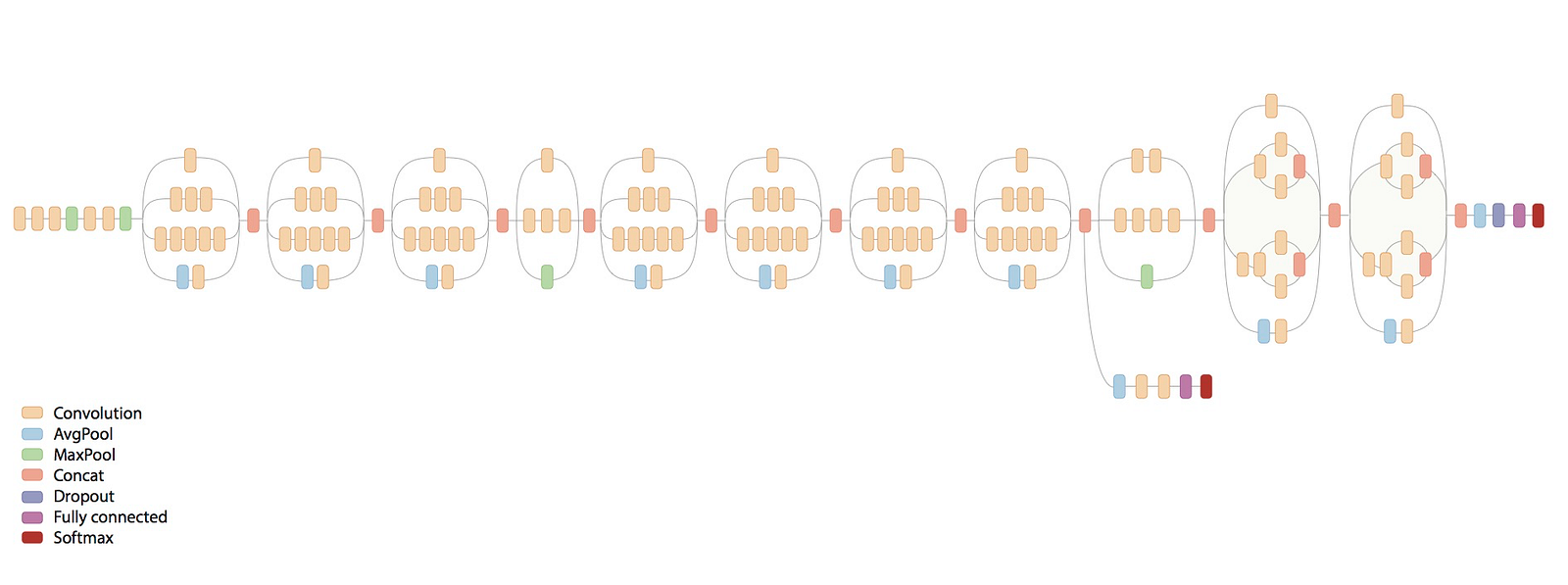
The previously illegible network architecture graphs are now seemingly approachable.

Concretely, the reading of Adrian Rosebrock’s book gave me the insight to decode the box-line diagrams of machine learning algorithms. The breakdown of a deep learning network architecture is now somewhat understandable. I am also familiar with the datasets (MNIST, CIFAR-10, and ImageNet) that are commonly used to benchmark various image recognition models, as well as the differences between image recognition models (such as VGG-16, Inception, etc).

Timing — Public Funding

One reason I decided machine learning and computer vision are important to learn now is related to a concept I learned from the book: Areas with heavy government investment in research are on track to have huge innovation. Currently, there are hundreds of millions of dollars being spent on research programs in the form of grants and scholarships, in addition to the specific funding being allocated to programs for specific machine learning related projects.

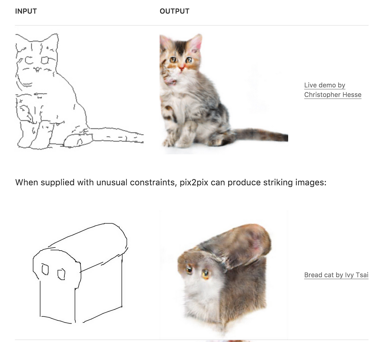
Example of pix2pix algorithm applied to “cat-ness”. https://distill.pub/2017/aia/

In addition to government spending, publicly accessible research from private institutions seems to be growing. The forms of research that currently exist, coming out of big tech companies and public foundations, are pushing forward the entire field of machine learning. I personally have never seen the same concentration of public projects funded by private institutions in the form of publications like distill.pub and collectives like the OpenAI foundation. The work they are putting out is unmatched.

Actionable tasks

Reviewing the materials I have been reading, I realize my memory is already failing me. I’m going to do more action-oriented reading from this point forward. I have a box with GPUs to work with now, so I don’t feel any limitations around training models and working on datasets.

Most recently, I attended a great conference on Spatial Data Science, hosted by Carto. There, I became very aware of how much I don’t know in the field of spatial data science. Before the conference, I was just calling the entire field “map location data stuff”.

Most recently, I attended a great conference on Spatial Data Science, hosted by Carto. Through the process, I am made very aware of how much I don’t know in the field of spatial data science. Before the conference, I was just calling the entire field “map location data stuff”.

I’ll continue making efforts to meet up with different people I find online with similar interests. I’ve already been able to do this with folks I find who live in New York and have written Medium posts relevant to my current search. Most recently, when exploring how to build a GPU box, I was able to meet a fellow machine learning explorer for breakfast.

By the middle of January, I’d like to be familiar with technical frameworks for training a model around graffiti images. I think at the very least, I want to have a set of images to work with, labels to associate the images to, and a process for cross-checking an unindexed image against the trained labels.


Thanks to Jihii Jolly for correcting my grammar.

Posted by uniqueone
,
https://m.facebook.com/groups/255834461424286?view=permalink&id=572281386446257

머신러닝 입문하시는 분들을 위해 흥미로운 사이트를 공유합니다. 나온지 좀 된거 같은데 Tensorflow KR에서 검색해 봐도 공유된 적이 없는것 같더군요. 혹시 한분이라도 보시고 도움되면 좋을 것 같아서 써요.

Intel AI Academy 에서 무료로 공개한 Machine Learning 101, Deep Learning 101 수업 입니다. Regression / Classification 부터 CNN RNN까지 다룬걸 보니 김성훈 교수님 수업이랑 오버랩 되네요. 복습한다고 생각하시고 보는것도 나쁘지 않을 것 같습니다.

PDF, 샘플코드, 동영상 조금으로 이루어져 있는데 깔끔하게 잘 만든것 같습니다. 코드는 keras를 사용합니다.

https://software.intel.com/en-us/ai-academy/students/kits
Posted by uniqueone
,
https://www.facebook.com/MachineLearningMastery/posts/1979228055625051

How to Visualize a Deep Learning Neural Network Model in Keras https://machinelearningmastery.com/visualize-deep-learning-neural-network-model-keras/
Posted by uniqueone
,
https://m.facebook.com/groups/255834461424286?view=permalink&id=570463146628081

다들 아시는 정보이시겠지만, 과제를 준비하면서 사용하였던 colorization, google deepdream, style transfer, matting 알고리즘에 대해 간단히 정리해보았습니다. (논문 + 코드 링크 정리입니다.)

올라오는 글들을 보면서 공부에 대해 자극도 많이 받고, 많은 정보를 얻어갑니다. 다들 감사합니다. 부족하지만 조금이나마 도움이 되었으면 합니다. (오류가 있다면 말씀부탁드리겠습니다.)

1. Colorization
(1) Colourful Image Colorization (Zhang et al. 2016)
   Link: http://richzhang.github.io/colorization/
(2) Automatic Colorization of Grayscale Images from Stanford cs229 class
   Description: http://cs229.stanford.edu/proj2013/KabirzadehSousaBlaes-AutomaticColorizationOfGrayscaleImages.pdf
   Code: https://github.com/prblaes/ImageColorization

2. Google deepdream
(1) (For Docker user) https://github.com/VISIONAI/clouddream
(2) (For Python user) https://www.pyimagesearch.com/2015/07/06/bat-country-an-extendible-lightweight-python-package-for-deep-dreaming-with-caffe-and-convolutional-neural-networks/
(3) (For IPython Notebook user) https://github.com/google/deepdream

3. Style Transfer
(1) Deep Photo style transfer (2017)
    paper: https://arxiv.org/abs/1703.07511
    code: https://github.com/luanfujun/deep-photo-styletransfer

4. Matting (Background removal and replacement)
(1) Deep Image Matting (Xu et al. 2017)
    paper: https://arxiv.org/abs/1703.03872
    code: https://github.com/Joker316701882/Deep-Image-Matting

(2) Scribble method
   1) paper: (Wang and Cohen 2005) An Iterative Optimization Approach for Unified Image Segmentation and Matting
   2) paper: (Levin et al. 2008) A Closed-Form Solution to Natural
Image Matting
      code: http://www.alphamatting.com/code.php

(3) Grabcut Method (Rother et al. 2004)
   paper: https://dl.acm.org/citation.cfm?id=1015720
   code: (based on opencv) https://docs.opencv.org/3.1.0/d8/d83/tutorial_py_grabcut.html

Posted by uniqueone
,

How much mathematics does an IT engineer need to learn to get into data science/machine learning?
https://towardsdatascience.com/how-much-maths-does-an-it-engineer-need-to-learn-to-get-into-data-science-machine-learning-7d6a42f79516

Homepage
Towards Data Science
Get started
HOMEDATA SCIENCEMACHINE LEARNINGPROGRAMMINGVISUALIZATIONEVENTSLETTERSCONTRIBUTE
Go to the profile of Tirthajyoti Sarkar
Tirthajyoti Sarkar
Semiconductor technologist, machine learning/data science zealot, Ph.D. in EE, blogger and writer.
Aug 29
How much mathematics does an IT engineer need to learn to get into data science/machine learning?

Disclaimer and Prologue
First, the disclaimer, I am not an IT engineer :-) I work in the field of semiconductors, specifically high-power semiconductors, as a technology development engineer, whose day job consists of dealing primarily with semiconductor physics, finite-element simulation of silicon fabrication process, or electronic circuit theory. There are, of course, some mathematics in this endeavor, but for better of worse, I don’t need to dabble in the kind of mathematics that will be necessary for a data scientist.
However, I have many friends in IT industry and observed a great many traditional IT engineers enthusiastic about learning/contributing to the exciting field of data science and machine learning/artificial intelligence. I am dabbling myself in this field to learn some tricks of the trade which I can apply to the domain of semiconductor device or process design. But when I started diving deep into these exciting subjects (by self-study), I discovered quickly that I don’t know/only have a rudimentary idea about/ forgot mostly what I studied in my undergraduate study some essential mathematics. In this LinkedIn article, I ramble about it…
Now, I have a Ph.D. in Electrical Engineering from a reputed US University and still I felt incomplete in my preparation for having solid grasp over machine learning or data science techniques without having a refresher in some essential mathematics. Meaning no disrespect to an IT engineer, I must say that the very nature of his/her job and long training generally leave him/her distanced from the world of applied mathematics. (S)he may be dealing with lot of data and information on a daily basis but there may not be an emphasis on rigorous modeling of that data. Often, there is immense time pressure, and the emphasis is on ‘use the data for your immediate need and move on’ rather than on deep probing and scientific exploration of the same. Unfortunately, data science should always be about the science (not data), and following that thread, certain tools and techniques become indispensable.
These tools and techniques — modeling a process (physical or informational) by probing the underlying dynamics, rigorously estimating the quality of the data source, training one’s sense for identification of the hidden pattern from the stream of information, or understanding clearly the limitation of a model— are the hallmarks of sound scientific process.
They are often taught at advanced graduate level courses in an applied science/engineering discipline. Or, one can imbibe them through high-quality graduate-level research work in similar field. Unfortunately, even a decade long career in traditional IT (devOps, database, or QA/testing) will fall short of rigorously imparting this kind of training. There is, simply, no need.
The Times They Are a-Changin’
Until now.
You see, in most cases, having impeccable knowledge of SQL queries, a clear sense of the overarching business need, and idea about the general structure of the corresponding RDBMS is good enough to perform the extract-transform-load cycle and thereby generating value to the company for any IT engineer worth his/her salt. But what happens if someone drops by and starts asking weird question like “is your artificially synthesized test data set random enough” or “how would you know if the next data point is within 3-sigma limit of the underlying distribution of your data”? Or, even the occasional quipping from the next-cubicle computer science graduate/nerd that the computational load for any meaningful mathematical operation with a table of data (aka a matrix) grows non-linearly with the size of table i.e. number of rows and columns, can be exasperating and confusing.
And these type of questions are growing in frequency and urgency, simply because data is the new currency.
Executives, technical managers, decision-makers are not satisfied anymore with just the dry description of a table, obtained by traditional ETL tools. They want to see the hidden pattern, they yarn to feel the subtle interaction between the columns, they would like to get the full descriptive and inferential statistics that may help in predictive modeling and extending the projection power of the data set far beyond the immediate range of values that it contains.
Today’s data must tell a story, or, sing a song if you like. However, to listen to its beautiful tune, one must be versed in the fundamental notes of the music, and those are mathematical truths.
Without much further ado, let us come to the crux of the matter. What are the essential topics/sub-topics of mathematics, that an average IT engineer must study/refresh if (s)he wants to enter into the field of business analytics/data science/data mining? I’ll show my idea in the following chart.

Basic Algebra, Functions, Set theory, Plotting, Geometry

Always a good idea to start at the root. Edifice of modern mathematics is built upon some key foundations — set theory, functional analysis, number theory etc. From an applied mathematics learning point of view, we can simplify studying these topics through some concise modules (in no particular order):

a) set theory basics, b) real and complex numbers and basic properties, c) polynomial functions, exponential, logarithms, trigonometric identities, d) linear and quadratic equations, e) inequalities, infinite series, binomial theorem, f) permutation and combination, g) graphing and plotting, Cartesian and polar co-ordinate systems, conic sections, h) basic geometry and theorems, triangle properties.
Calculus
Sir Issac Newton wanted to explain the behavior of heavenly bodies. But he did not have a good enough mathematical tool to describe his physical concepts. So he invented this (or a certain modern form) branch of mathematics when he was hiding away on his countryside farm from the plague outbreak in urban England. Since then, it is considered the gateway to advanced learning in any analytical study — pure or applied science, engineering, social science, economics, …

Not surprisingly then, the concept and application of calculus pops up in numerous places in the field of data science or machine learning. Most essential topics to be covered are as follows -
a) Functions of single variable, limit, continuity and differentiability, b) mean value theorems, indeterminate forms and L’Hospital rule, c) maxima and minima, d) product and chain rule, e) Taylor’s series, f) fundamental and mean value-theorems of integral calculus, g) evaluation of definite and improper integrals, h) Beta and Gamma functions, i) Functions of two variables, limit, continuity, partial derivatives, j) basics of ordinary and partial differential equations.
Linear Algebra
Got a new friend suggestion on Facebook? A long lost professional contact suddenly added you on LinkedIn? Amazon suddenly recommended an awesome romance-thriller for your next vacation reading? Or Netflix dug up for you that little-known gem of a documentary which just suits your taste and mood?

Doesn’t it feel good to know that if you learn basics of linear algebra, then you are empowered with the knowledge about the basic mathematical object that is at the heart of all these exploits by the high and mighty of the tech industry?
At least, you will know the basic properties of the mathematical structure that controls what you shop on Target, how you drive using Google Map, which song you listen to on Pandora, or whose room you rent on Airbnb.
The essential topics to study are (not an ordered or exhaustive list by any means):
a) basic properties of matrix and vectors —scalar multiplication, linear transformation, transpose, conjugate, rank, determinant, b) inner and outer products, c) matrix multiplication rule and various algorithms, d) matrix inverse, e) special matrices — square matrix, identity matrix, triangular matrix, idea about sparse and dense matrix, unit vectors, symmetric matrix, Hermitian, skew-Hermitian and unitary matrices, f) matrix factorization concept/LU decomposition, Gaussian/Gauss-Jordan elimination, solving Ax=b linear system of equation, g) vector space, basis, span, orthogonality, orthonormality, linear least square, h) singular value decomposition, i) eigenvalues, eigenvectors, and diagonalization.
Here is a nice Medium article on what you can accomplish with linear algebra.
Statistics and Probability
Only death and taxes are certain, and for everything else there is normal distribution.

The importance of having a solid grasp over essential concepts of statistics and probability cannot be overstated in a discussion about data science. Many practitioners in the field actually call machine learning nothing but statistical learning. I followed the widely known “An Introduction to Statistical Learning” while working on my first MOOC in machine learning and immediately realized the conceptual gaps I had in the subject. To plug those gaps, I started taking other MOOCs focused on basic statistics and probability and reading up/watching videos on related topics. The subject is vast and endless, and therefore focused planning is critical to cover most essential concepts. I am trying to list them as best as I can but I fear this is the area where I will fall short by most amount.
a) data summaries and descriptive statistics, central tendency, variance, covariance, correlation, b) Probability: basic idea, expectation, probability calculus, Bayes theorem, conditional probability, c) probability distribution functions — uniform, normal, binomial, chi-square, student’s t-distribution, central limit theorem, d) sampling, measurement, error, random numbers, e) hypothesis testing, A/B testing, confidence intervals, p-values, f) ANOVA, g) linear regression, h) power, effect size, testing means, i) research studies and design-of-experiment.
Here is a nice article on the necessity of statistics knowledge for a data scientist.
Special Topics: Optimization theory, Algorithm analysis
These topics are little different from the traditional discourse in applied mathematics as they are mostly relevant and most widely used in specialized fields of study — theoretical computer science, control theory, or operation research. However, a basic understanding of these powerful techniques can be so fruitful in the practice of machine learning that they are worth mentioning here.

For example, virtually every machine learning algorithm/technique aims to minimize some kind of estimation error subject to various constraints. That, right there, is an optimization problem, which is generally solved by linear programming or similar techniques. On the other hand, it is always deeply satisfying and insightful experience to understand a computer algorithm’s time complexity as it becomes extremely important when the algorithm is applied to a large data set. In this era of big data, where a data scientist is routinely expected to extract, transform, and analyze billions of records, (s)he must be extremely careful about choosing the right algorithm as it can make all the difference between amazing performance or abject failure. General theory and properties of algorithms are best studied in a formal computer science course but to understand how their time complexity (i.e. how much time the algorithm will take to run for a given size of data) is analyzed and calculated, one must have rudimentary familiarity with mathematical concepts such as dynamic programming or recurrence equations. A familiarity with the technique of proof by mathematical induction can be extremely helpful too.
Epilogue
Scared? Mind-bending list of topics to learn just as per-requisite? Fear not, you will learn on the go and as needed. But the goal is to keep the windows and doors of your mind open and welcoming.
There is even a concise MOOC course to get you started. Note, this is a beginner-level course for refreshing your high-school or freshman year level knowledge. And here is a summary article on 15 best math courses for data science on kdnuggets.
But you can be assured that, after refreshing these topics, many of which you may have studied in your undergraduate, or even learning new concepts, you will feel so empowered that you will definitely start to hear the hidden music that the data sings. And that’s called a big leap towards becoming a data scientist…
#datascience, #machinelearning, #information, #technology, #mathematics
If you have any questions or ideas to share, please contact the author at tirthajyoti[AT]gmail.com. Also you can check author’s GitHub repositories for other fun code snippets in Python, R, or MATLAB and machine learning resources. You can also follow me on LinkedIn.
Machine LearningData ScienceMathematicsStatisticsLinear Algebra
One clap, two clap, three clap, forty?
By clapping more or less, you can signal to us which stories really stand out.


81

Follow
Go to the profile of Tirthajyoti Sarkar
Tirthajyoti Sarkar
Semiconductor technologist, machine learning/data science zealot, Ph.D. in EE, blogger and writer.
Follow
Towards Data Science
Sharing concepts, ideas, and codes.
More on Statistics from Towards Data Science
The 10 Statistical Techniques Data Scientists Need to Master
Go to the profile of James Le
James Le

8.3K

Also tagged Statistics
Should you write about real goals or expected goals? A guide for journalists.
Go to the profile of David Sumpter
David Sumpter

27

Related reads
How to choose effective MOOCs for machine learning and data science?
Go to the profile of Tirthajyoti Sarkar
Tirthajyoti Sarkar

422
Posted by uniqueone
,
https://m.facebook.com/groups/255834461424286?view=permalink&id=565488850458844

딥러닝의 내부에서 일어나는 일을 Information Theory로, 그 중에서도 Information Bottleneck 이라는 원리로 접근하는 이론에 관한 글입니다.
한마디로 딥러닝 아키텍쳐안의 노드는 바틀넥처럼 작용하여 자기에게 들어온 인포메이션 중 미래의 목표와 관련된 것들만을 선별하고 그 나머지는 버림으로서 (여기서는 compression이라 표현) 일반화라는 목표에 도달하게 된다는 것입니다. 
즉 개냐 고양이냐 0이냐 1이냐 하는 식으로 일반화하는 데에 필요한 정보들만 계속 추상화되어 바틀넥안으로 밀어넣어진다는 것인데 이 과정에서 인풋에 들어있는 얼마나 많은 정보들이 걸러지고 버려지겠는지만 생각해보아도 딥러닝의 파워를 한 번에 느껴볼 수가 있어요. 다시말해 입력의 세부 정보들은 모두 압축되고 혹은 날아가고 기다 아니다, 이거다 저거다만 남는 것이니 러닝의 가장 중요한 부분은 버리는데서 이루어진다는 것. 쿨!

이 이론을 발표한 이스라엘의 히브루 대학의 물리학 교수인 Naftali Tishby는 자신이 수십년간 연구해온 이 인포메이션 바틀넥 원리라는 주제를 최근 성공적으로 딥러닝의 내부 작용의 원리와 연관을 시켜내었습니다. 이 기사에서 보면 딥러닝의 대부인 힌튼교수도 그의 유튜브 동영상 강연을 보고는 잘 이해하기는 어렵지만 딥러닝 내부 원리를 설명하는 좋은 이론인 거 같다며 Tishby의 연구 결과에 찬사를 보냈다고 하네요. *힌튼교수가 보았다는 그의 동영상 강의는 여기. https://www.youtube.com/watch?v=bLqJHjXihK8&t=2234s

P.S.: 며칠전에 여기에 딥러닝의 블랙박스라는게 뭘 모른다고 하는거냐고 툭 묻듯이 한 줄 썼는데 관심 가져주신 분들 감사합니다. ^^ 
Tishby교수의 동영상 강연은 심도가 있는 반면 매우 테크니컬한 면이 있어서 이해하기에 어려운 점이 있었는데 이 기사는 영문이지만 읽기에 크게 어렵지 않아 이 글을 공유합니다.

https://www.wired.com/story/new-theory-deep-learning/?mbid=social_fb_onsiteshare
Posted by uniqueone
,
https://m.facebook.com/groups/107107546348803?view=permalink&id=532112330514987

TensorFlow Speech Recognition - Kaggle competition is going on. I wrote a basic tutorial on speech (word) recognition using some of the datasets from the competition.
.
Hope it will be helpful for some of you. Thanks in advance for reading!
.

https://blog.manash.me/building-a-dead-simple-word-recognition-engine-using-convnet-in-keras-25e72c19c12b
Posted by uniqueone
,

Kaggle-knowhow/README.md at master · zzsza/Kaggle-knowhow · GitHub
https://github.com/zzsza/Kaggle-knowhow/blob/master/README.md
Posted by uniqueone
,

Probabilistic Graphical Models Tutorial — Part 2 – Stats and Bots
https://blog.statsbot.co/probabilistic-graphical-models-tutorial-d855ba0107d1


Homepage
Stats and Bots
Get started
HOMEDATA SCIENCEANALYTICSSTARTUPSBOTSDESIGNSUBSCRIBE TRY STATSBOT FREE
Go to the profile of Prasoon Goyal
Prasoon Goyal
PhD candidate at UT Austin. For more content on machine learning by me, check my Quora profile (https://www.quora.com/profile/Prasoon-Goyal).
Nov 23
Probabilistic Graphical Models Tutorial — Part 2
Parameter estimation and inference algorithms

In the previous part of this probabilistic graphical models tutorial for the Statsbot team, we looked at the two types of graphical models, namely Bayesian networks and Markov networks. We also explored the problem setting, conditional independences, and an application to the Monty Hall problem. In this post, we will cover parameter estimation and inference, and look at another application.

Parameter Estimation
Bayesian networks
Estimating the numbers in the CPD tables of a Bayesian network simply amounts to counting how many times that event occurred in our training data. That is, to estimate p(SAT=s1 | Intelligence = i1), we simply count the fraction of data points where SAT=s1 and Intelligence = i1, out of the total data points where Intelligence = i1. While this approach may appear ad hoc, it turns out that the parameters so obtained maximize the likelihood of the observed data.
Markov networks
For Markov networks, unfortunately, the above counting approach does not have a statistical justification (and will therefore lead to suboptimal parameters). So, we need to use more sophisticated techniques. The basic idea behind most of these techniques is gradient descent — we define parameters that describe the probability distribution, and then use gradient descent to find values for these parameters that maximize the likelihood of the observed data.
Finally, now that we have the parameters of our model, we want to use them on new data, to perform inference!
Inference
The bulk of the literature in probabilistic graphical models focuses on inference. The reasons are two-fold:
Inference is why we came up with this entire framework — being able to make predictions from what we already know.
Inference is computationally hard! In some specific kinds of graphs, we can perform inference fairly efficiently, but on general graphs, it is intractable. So we need to use approximate algorithms that trade off accuracy for efficiency.
There are several questions we can answer with inference:
Marginal inference: Finding the probability distribution of a specific variable. For instance, given a graph with variables A, B, C, and D, where A takes values 1, 2, and 3, find p(A=1), p(A=2) and p(A=3).
Posterior inference: Given some observed variables v_E (E for evidence) that take values e, finding the posterior distribution p(v_H | v_E=e) for some hidden variables v_H.
Maximum-a-posteriori (MAP) inference: Given some observed variables v_E that take values e, finding the setting of other variables v_H that have the highest probability.
Answers to these questions may be useful by themselves, or may need to be used as part of larger tasks.
In what follows, we are going to look at some of the popular algorithms for answering these questions, both exact and approximate. All these algorithms are applicable on both Bayesian networks and Markov networks.
Variable Elimination
Using the definition of conditional probability, we can write the posterior distribution as:

Let’s see how we can compute the numerator and the denominator above, using a simple example. Consider a network with three variables, and the joint distribution defined as follows:

Let’s say we want to compute p(A | B=1). Note that this means that we want to compute the values p(A=0 | B=1)and p(A=1 | B=1), which should sum to one. Using the above equation, we can write

The numerator is the probability that A = 0 and B = 1. We don’t care about the values of C. So we would sum over all the values of C. (This comes from basic probability — p(A=0, B=1, C=0) and p(A=0, B=1, C=1) are mutually exclusive events, so their union p(A = 0, B=1) is just the sum of the individual probabilities.)
So we add rows 3 and 4 to get p(A=0, B=1) = 0.15. Similarly, adding rows 7 and 8 gives usp(A=1, B=1) = 0.40. Also, we can compute the denominator by summing over all rows that contain B=1, that is, rows 3, 4, 7, and 8, to get p(B=1) = 0.55. This gives us the following:
p(A = 0 | B = 1) = 0.15 / 0.55 = 0.27
p(A = 1 | B = 1) = 0.40 / 0.55 = 0.73
If you look at the above computation closely, you would notice that we did some repeated computations — adding rows 3 & 4, and 7 & 8 twice. A more efficient way to compute p(B=1)would have been to simply add the values p(A=0, B=1) and p(A=1, B=1). This is the basic idea of variable elimination.
In general, when you have a lot of variables, not only can you use the values of the numerator to compute the denominator, but the numerator by itself will contain repeated computations, if evaluated naively. You can use dynamic programming to use precomputed values efficiently.
Because we are summing over one variable at a time, thereby eliminating it, the process of summing out multiple variables amounts to eliminating these variables one at a time. Hence, the name “variable elimination.”
It is straightforward to extend the above process to solve the marginal inference or MAP inference problems as well. Similarly, it is easy to generalize the above idea to apply it to Markov networks too.
The time complexity of variable elimination depends on the graph structure, and the order in which you eliminate the variables. In the worst case, it has exponential time complexity.
Belief Propagation
The VE algorithm that we just saw gives us only one final distribution. Suppose we want to find the marginal distributions for all variables. Instead of running variable elimination multiple times, we can do something smarter.
Suppose you have a graph structure. To compute a marginal, you need to sum the joint distribution over all other variables, which amounts to aggregating information from the entire graph. Here’s an alternate way of aggregating information from the entire graph — each node looks at its neighbors, and approximates the distribution of variables locally.
Then, every pair of neighboring nodes send “messages” to each other where the messages contain the local distributions. Now, every node looks at the messages it receives, and aggregates them to update its probability distributions of variables.

In the figure above, C aggregates information from its neighbors A and B, and sends a message to D. Then, D aggregates this message with the information from E and F.
The advantage of this approach is that if you save the messages that you are sending at every node, one forward pass of messages followed by one backward pass gives all nodes information about all other nodes. That information can then be used to compute all the marginals, which was not possible in variable elimination.
If the graph does not contain cycles, then this process converges after a forward and a backward pass. If the graph contains cycles, then this process may or may not converge, but it can often be used to get an approximate answer.
Approximate inference
Because exact inference may be prohibitively time consuming for large graphical models, numerous approximate inference algorithms have been developed for graphical models, most of which fall into one of the following two categories:
Sampling-based
These algorithms estimate the desired probability using sampling. As a simple example, consider the following scenario — given a coin, how you would determine the probability of getting heads when the coin is tossed? The simplest thing is to flip the coin, say, 100 times, and find out the fraction of tosses in which you get heads.
This is a sampling-based algorithm to estimate the probability of heads. For more complex questions in probabilistic graphical models, you can use a similar procedure. Sampling-based algorithms can further be divided into two classes. In the first one, the samples are independent of each other, as in the coin toss example above. These algorithms are called Monte Carlo methods.
For problems with many variables, generating good quality independent samples is difficult, and therefore, we generate dependent samples, that is, each new sample is random, but close to the last sample. Such algorithms are called Markov Chain Monte Carlo (MCMC) methods, because the samples form a “Markov chain.” Once we have the samples, we can use them to answer various inference questions.
Variational methods
Instead of using sampling, variational methods try to approximate the required distribution analytically. Suppose you write out the expression for computing the distribution of interest — marginal probability distribution or posterior probability distribution.
Often, these expressions have summations or integrals in them that are computationally expensive to evaluate exactly. A good way to approximate these expressions is to then solve for an alternate expression, and somehow ensure that this alternate expression is close to the original expression. This is the basic idea behind variational methods.
When we are trying to estimate a complex probability distribution p_complex, we define a separate set of probability distributions P_simple, which are easier to work with, and then find the probability distribution p_approx from P_simple that is closest to p_complex.
Application: Image denoising
Let us now use some of the ideas we just discussed on a real problem. Let’s say you have the following image:

Now suppose that it got corrupted by random noise, so that your noisy image looks as follows:

The goal is to recover the original image. Let’s see how we can use probabilistic graphical models to do this.
The first step is to think about what our observed and unobserved variables are, and how we can connect them to form a graph. Let us define each pixel in the noisy image as an observed random variable, and each pixel in the ground truth image as an unobserved variable. So, if the image is M x N, then there are MN observed variables and MN unobserved variables. Let us denote observed variables as X_ij and unobserved variables as Y_ij. Each variable takes values +1 and -1 (corresponding to black and white pixels, respectively). Given the observed variables, we want to find the most likely values of the unobserved variables. This corresponds to MAP inference.
Now, let us use some domain knowledge to build the graph structure. Clearly, the observed variable at position (i, j) in the noisy image depends on the unobserved variable at position (i, j) in the ground truth image. This is because most of the time, they are identical.
What more can we say? For ground truth images, the neighboring pixels usually have the same values — this is not true at the boundaries of color change, but inside a single-colored region, this property holds. Therefore, we connect Y_ij and Y_kl if they are neighboring pixels.
So, our graph structure looks as follows:

Here, the white nodes denote the unobserved variables Y_ij and the grey nodes denote observed variables X_ij. Each X_ij is connected to the corresponding Y_ij, and each Y_ij is connected to its neighbors.
Note that this is a Markov network, because there is no cause-effect relation between pixels of an image, and therefore, defining directions of arrows in Bayesian networks is unnatural here.
Our MAP inference problem can be mathematically written as follows:

Here, we used some standard simplification techniques common in maximum log likelihood computation. We will use X and Y(without subscripts) to denote the collection of all X_ij and Y_ij values, respectively.
Now, we need to define our joint distribution P(X, Y) based on our graph structure. Let’s assume that P(X, Y) consists of two kinds of factors — ϕ(X_ij, Y_ij) and ϕ(Y_ij,Y_kl), corresponding to the two kinds of edges in our graph. Next, we define the factors as follows:
ϕ(X_ij, Y_ij) = exp(w_e X_ij Y_ij), where w_e is a parameter greater than zero. This factor takes large values when X_ij and Y_ij are identical, and takes small values when X_ij and Y_ij are different.
ϕ(Y_ij, Y_kl) = exp(w_s Y_ij Y_kl), where w_s is a parameter greater than zero, as before. This factor favors identical values of Y_ij and Y_kl.
Therefore, our joint distribution is given by:

where (i, j) and (k, l) in the second product are adjacent pixels, and Z is a normalization constant.
Plugging this into our MAP inference equation gives:

Note that we have dropped the term containing Zsince it does not affect the solution.
The values of w_e and w_s are obtained using parameter estimation techniques from pairs of ground truth and noisy images. This process is fairly mathematically involved (although, at the end of the day, it is just gradient descent on a complicated function), and therefore, we shall not delve into it here. We will assume that we have obtained the following values of these parameters — w_e = 8 and w_s = 10.
The main focus of this example will be inference. Given these parameters, we want to solve the MAP inference problem above. We can use a variant of belief propagation to do this, but it turns out that there is a much simpler algorithm called Iterated conditional modes (ICM) for graphs with this specific structure.
The basic idea is that at each step, you choose one node, Y_ij, look at the value of the MAP inference expression for both Y_ij = -1 and Y_ij = 1, and pick the one with the higher value. Repeating this process for a fixed number of iterations or until convergence usually works reasonably well.
You can use this Python code to do this for our model.
This is the denoised image returned by the algorithm:

Pretty good, isn’t it? Of course, you can use more fancy techniques, both within graphical models, and outside, to generate something better, but the takeaway from this example is that a simple Markov network with a simple inference algorithm already gives you reasonably good results.
Quantitatively, the noisy image has about 10% of the pixels that are different from the original image, while the denoised image produced by our algorithm has about 0.6% of the pixels that are different from the original image.
It is important to note that the graph that we used is fairly large — the image size is about 440 x 300, so the total number of nodes is close to 264,000. Therefore, exact inference in such models is essentially infeasible, and what we get out of most algorithms, including ICM, is a local optimum.
Let’s recap
In this section, let us briefly review the key concepts we covered in this two-part series:
Graphical models: A graphical model consists of a graph structure where nodes represent random variables and edges represent dependencies between variables.
Bayesian networks: These are directed graphical models, with a conditional probability distribution table associated with each node.
Markov networks: These are undirected graphical models, with a potential function associated with each clique.
Conditional independences: Based on how the nodes in the graph are connected, we can write conditional independence statements of the form “X is independent of Y given Z.”
Parameter estimation: Given some data and the graph structure, we want to fill the CPD tables or compute the potential functions.
Inference: Given a graphical model, we want to answer questions about unobserved variables. These questions are usually one of the following — Marginal inference, posterior inference, and MAP inference.
Inference on general graphical models is computationally intractable. We can divide inference algorithms into two broad categories — exact and approximate. Variable elimination and belief propagation in acyclic graphs are examples of exact inference algorithms. Approximate inference algorithms are necessary for large-scale graphs, and usually fall into sampling-based methods or variational methods.
Conclusions
We looked at some of the core ideas in probabilistic graphical models in this two-part tutorial. As you should be able to appreciate at this point, graphical models provide an interpretable way to model many real-world tasks, where there are dependencies. Using graphical models gives us a way to work on such tasks in a principled manner.
Before we close, it is important to point out that this tutorial, by no means, is complete — many details have been skipped to keep the content intuitive and simple. The standard textbook on probabilistic graphical models is over a thousand pages! This tutorial is meant to serve as a starting point, to get you interested in the field, so that you can look up more rigorous resources.
Here are some additional resources that you can use to dig deeper into the field:
Graphical Models in a Nutshell
Graphical Models textbook
You should also be able to find a few chapters on graphical models in standard machine learning textbooks.

YOU’D ALSO LIKE:
Probabilistic Graphical Models Tutorial — Part 1

Basic terminology and the problem setting
blog.statsbot.co
Machine Learning Algorithms: Which One to Choose for Your Problem

Intuition of using different kinds of algorithms in different tasks
blog.statsbot.co
Neural networks for beginners: popular types and applications

An introduction to neural networks learning
blog.statsbot.co
Machine LearningData ScienceAlgorithmsBayesian StatisticsMarkov Chains
One clap, two clap, three clap, forty?
By clapping more or less, you can signal to us which stories really stand out.


265

Follow
Go to the profile of Prasoon Goyal
Prasoon Goyal
PhD candidate at UT Austin. For more content on machine learning by me, check my Quora profile (https://www.quora.com/profile/Prasoon-Goyal).
Follow
Stats and Bots
Stats and Bots
Data stories on machine learning and analytics. From Statsbot’s makers.
More from Stats and Bots
Neural networks for beginners: popular types and applications
Go to the profile of Jay Shah
Jay Shah

287

Also tagged Markov Chains
Implementing Markov Chain in Swift. Generating Texts.
Go to the profile of Swift The Sorrow
Swift The Sorrow

41

More on Algorithms from Stats and Bots
Data Structures Related to Machine Learning Algorithms
Go to the profile of Peter Mills
Peter Mills

275
Posted by uniqueone
,

An Introduction to different Types of Convolutions in Deep Learning
https://towardsdatascience.com/types-of-convolutions-in-deep-learning-717013397f4d

Homepage
Towards Data Science
Get started
HOMEDATA SCIENCEMACHINE LEARNINGPROGRAMMINGVISUALIZATIONEVENTSLETTERSCONTRIBUTE
Go to the profile of Paul-Louis Pröve
Paul-Louis Pröve
Artificial Intelligence @ PwC
Jul 22
An Introduction to different Types of Convolutions in Deep Learning

Let me give you a quick overview of different types of convolutions and what their benefits are. For the sake of simplicity, I’m focussing on 2D convolutions only.
Convolutions
First we need to agree on a few parameters that define a convolutional layer.

2D convolution using a kernel size of 3, stride of 1 and padding
Kernel Size: The kernel size defines the field of view of the convolution. A common choice for 2D is 3 — that is 3x3 pixels.
Stride: The stride defines the step size of the kernel when traversing the image. While its default is usually 1, we can use a stride of 2 for downsampling an image similar to MaxPooling.
Padding: The padding defines how the border of a sample is handled. A (half) padded convolution will keep the spatial output dimensions equal to the input, whereas unpadded convolutions will crop away some of the borders if the kernel is larger than 1.
Input & Output Channels: A convolutional layer takes a certain number of input channels (I) and calculates a specific number of output channels (O). The needed parameters for such a layer can be calculated by I*O*K, where K equals the number of values in the kernel.
Dilated Convolutions
(a.k.a. atrous convolutions)

2D convolution using a 3 kernel with a dilation rate of 2 and no padding
Dilated convolutions introduce another parameter to convolutional layers called the dilation rate. This defines a spacing between the values in a kernel. A 3x3 kernel with a dilation rate of 2 will have the same field of view as a 5x5 kernel, while only using 9 parameters. Imagine taking a 5x5 kernel and deleting every second column and row.
This delivers a wider field of view at the same computational cost. Dilated convolutions are particularly popular in the field of real-time segmentation. Use them if you need a wide field of view and cannot afford multiple convolutions or larger kernels.
Transposed Convolutions
(a.k.a. deconvolutions or fractionally strided convolutions)
Some sources use the name deconvolution, which is inappropriate because it’s not a deconvolution. To make things worse deconvolutions do exists, but they’re not common in the field of deep learning. An actual deconvolution reverts the process of a convolution. Imagine inputting an image into a single convolutional layer. Now take the output, throw it into a black box and out comes your original image again. This black box does a deconvolution. It is the mathematical inverse of what a convolutional layer does.
A transposed convolution is somewhat similar because it produces the same spatial resolution a hypothetical deconvolutional layer would. However, the actual mathematical operation that’s being performed on the values is different. A transposed convolutional layer carries out a regular convolution but reverts its spatial transformation.

2D convolution with no padding, stride of 2 and kernel of 3
At this point you should be pretty confused, so let’s look at a concrete example. An image of 5x5 is fed into a convolutional layer. The stride is set to 2, the padding is deactivated and the kernel is 3x3. This results in a 2x2 image.
If we wanted to reverse this process, we’d need the inverse mathematical operation so that 9 values are generated from each pixel we input. Afterward, we traverse the output image with a stride of 2. This would be a deconvolution.

Transposed 2D convolution with no padding, stride of 2 and kernel of 3
A transposed convolution does not do that. The only thing in common is it guarantees that the output will be a 5x5 image as well, while still performing a normal convolution operation. To achieve this, we need to perform some fancy padding on the input.
As you can imagine now, this step will not reverse the process from above. At least not concerning the numeric values.
It merely reconstructs the spatial resolution from before and performs a convolution. This may not be the mathematical inverse, but for Encoder-Decoder architectures, it’s still very helpful. This way we can combine the upscaling of an image with a convolution, instead of doing two separate processes.
Separable Convolutions
In a separable convolution, we can split the kernel operation into multiple steps. Let’s express a convolution as y = conv(x, k) where y is the output image, x is the input image, and k is the kernel. Easy. Next, let’s assume k can be calculated by: k = k1.dot(k2). This would make it a separable convolution because instead of doing a 2D convolution with k, we could get to the same result by doing 2 1D convolutions with k1 and k2.

Sobel X and Y filters
Take the Sobel kernel for example, which is often used in image processing. You could get the same kernel by multiplying the vector [1, 0, -1] and [1,2,1].T. This would require 6 instead of 9 parameters while doing the same operation.
The example above shows what’s called a spatial separable convolution, which to my knowledge isn’t used in deep learning. I just wanted to make sure you don’t get confused when stumbling upon those. In neural networks, we commonly use something called a depthwise separable convolution.
This will perform a spatial convolution while keeping the channels separate and then follow with a depthwise convolution. In my opinion, it can be best understood with an example.
Let’s say we have a 3x3 convolutional layer on 16 input channels and 32 output channels. What happens in detail is that every of the 16 channels is traversed by 32 3x3 kernels resulting in 512 (16x32) feature maps. Next, we merge 1 feature map out of every input channel by adding them up. Since we can do that 32 times, we get the 32 output channels we wanted.
For a depthwise separable convolution on the same example, we traverse the 16 channels with 1 3x3 kernel each, giving us 16 feature maps. Now, before merging anything, we traverse these 16 feature maps with 32 1x1 convolutions each and only then start to them add together. This results in 656 (16x3x3 + 16x32x1x1) parameters opposed to the 4608 (16x32x3x3) parameters from above.
The example is a specific implementation of a depthwise separable convolution where the so called depth multiplier is 1. This is by far the most common setup for such layers.
We do this because of the hypothesis that spatial and depthwise information can be decoupled. Looking at the performance of the Xception model this theory seems to work. Depthwise separable convolutions are also used for mobile devices because of their efficient use of parameters.
Questions?
This concludes our little tour through different types of convolutions. I hope it helped to get a brief overview of the matter. Drop a comment if you have any remaining questions and check out this GitHub page for more convolution animations.
Machine LearningConvolutionalCnnNeural NetworksDeep Learning
One clap, two clap, three clap, forty?
By clapping more or less, you can signal to us which stories really stand out.


572
5
Follow
Go to the profile of Paul-Louis Pröve
Paul-Louis Pröve
Medium member since Oct 2017
Artificial Intelligence @ PwC
Follow
Towards Data Science
Sharing concepts, ideas, and codes.
More from Towards Data Science
Making Your Own Spotify Discover Weekly Playlist
Go to the profile of Nick Behrens
Nick Behrens

1.4K

Also tagged Neural Networks
Yes you should understand backprop
Go to the profile of Andrej Karpathy
Andrej Karpathy

4.4K

Related reads
Using GANS for semi-supervised learning
In supervised learning, we have a training set of inputs x and class labels y. We train a model that takes x as input and gives y as output…
Go to the profile of Manish Chablani
Manish Chablani

34

Responses
Conversation between Krishna Teja and Paul-Louis Pröve.
Go to the profile of Krishna Teja
Krishna Teja
Sep 18
Hi Paul,
It’s a great post. I would like to add a bit to your explanation on usage of separable convolutions in neural networks.
Note: In neural networks a 2D convolution has 3 dimensions such as height, width and depth where the depth is always equivalent to the number of input channels. For example…
Read more…

8
1 response
Go to the profile of Paul-Louis Pröve
Paul-Louis Pröve
Oct 16
Krishna, thank you so much for taking the time and showing the details of the actual tensor transformations. When you use high level frameworks such as Keras you never touch this functional level. I have a couple of questions:
Are you aware of any papers using spatial separable convolutions in deep learning? It sounds like a…
Posted by uniqueone
,
역시나 래블업에서 다른 작업중에 파생된 결과물을 공개합니다.

구글에서 공개한 머신러닝 용어집 (https://developers.google.com/machine-learning/glossary/) 을 번역한 글입니다. TensorFlow 및 케라스 온라인 강의/실습을 준비하며 용어 통일 및 참조용으로 만든 글인데, 고칠 부분에 대해 피드백을 받을 겸 먼저 공개해 봅니다.

많은 도움이 되셨으면 합니다.

덧) 고수님들께 피드백도 많이 부탁 드립니다!
덧2) 가능하면 연말까지는 하루에 하나씩 backend.AI 및 코드온웹의 파생 결과물들을 공개해 보겠습니다!

https://www.codeonweb.com/@mookiekim/ml-glossary
Posted by uniqueone
,

Top 10 Videos on Deep Learning in Python
https://www.kdnuggets.com/2017/11/top-10-videos-deep-learning-python.html?utm_content=buffer765d8&utm_medium=social&utm_source=facebook.com&utm_campaign=buffer


This ‘Top 10’ list has been created on the basis of best content, and not exactly the number of views. To help you choose an appropriate framework, we first start with a video that compares few of the popular Python DL libraries. I have included the highlights and my views on the pros and cons of each of these 10 items, so you can choose one that best suits your needs. I have saved the best for last- the most comprehensive yet free YouTube course on DL ☺. Let’s begin!

1. Overview: Deep Learning Frameworks compared (96K views) - 5 minutes

Before I actually list the best DL in Python videos, it is important that one understands the differences between the 5 most popular deep learning frameworks -SciKit Learn, TensorFlow, Theano, Keras, and Caffe. This 5 minute video by Siraj Raval gives you the best possible comparison between the pros and cons of each framework and even presents the structure of code samples to help you better decide. Start with this.

2. Playlist: TensorFlow tutorial by Sentdex (114 K views) - 4.5 hours

This playlist of 14 videos by Sentdex is the most well-organized, thoroughly explained ,concise yet easy to follow tutorial on Deep Learning in Python. It includes TensorFlow implementation of a Recurrent Neural Network and Convolutional Neural Network with the MNIST dataset.

3. Individual tutorial: TensorFlow tutorial 02: Convolutional Neural Network (69.7 K views) - 36 minutes

This tutorial by Magnus Pedersen on the YouTube channel Hvass Laboratories, is worth its weight in gold- excellent comments in the code; plus, the instructor speaks without interruption. Watch this video to understand scripts in TensorFlow. Thank me later☺

4. Overview : How to predict stock prices easily (210 K views) - 9 minutes

In this video, Siraj Raval uses a special type of recurrent neural network called an LSTM network. He uses the Keras library with a TensorFlow backend. He explains the reason behind using recurrent nets for time series data and later, uses it to predict the daily closing price of the S&P 500 based on training data for 16 years. The link to the Github code is given in its description box.

5. Tutorial: Introduction to Deep Learning with Python and the Theano library (201 K views) - 52 minutes

If you want a talk on Python with the Theano library in under an hour, targeted towards beginners, then you can refer to this talk by Alec Radford. Unlike most other talks on this topic, this one compares the features of an ‘old’ net versus a ‘modern’ net, ie nets prior to 2000 versus nets post-2012.

6. Playlist: PyTorch Zero to All (3 K views) - 2 hours 15 minutes

In this series of 11 videos, Sung Kim teaches you PyTorch from the ground up. A highlight of this series is Lecture 10, where he teaches you to build a basic CNN with detailed emphasis of understanding the concept of CNN’s using his detailed diagrams.

7. Individual tutorial: TensorFlow tutorial (43.9 K views) - 49 minutes

This single tutorial by Edureka implements DL using TensorFlow. It is a very good tutorial for beginners in TensorFlow. It teaches TensorFlow basics and data structures. It also includes a usecase for using DL as a Naval Mine identifier- to identify whether an underwater obstacle is a rock or a mine.

8. Playlist: Deep Learning with Python (1.8K views) - 83 minutes

The YouTube channel ‘Machine Learning TV‘ has published a series of 15 videos totaling 83 minutes using Theano and Keras to use DL for automatic image captioning. It shows you how to train your first deep neural net for classifying digits from the MNIST dataset. It also has a good explanation on loading and reusing pre-trained models in Theano.

9. Playlist: Deep Learning with Keras- Python (30.3 K views) - 85 minutes

The YouTube channel ‘The SemiColon‘ has published a series of 11 videos on tutorials using Theano and Keras to implement a chatbot using DL. It includes explanations on Convolutional Neural Network, Recurrent Neural Network in Theano with Keras, Neural Networks and Backpropagation in scikit-learn library on the handwriting recognition (MNIST) dataset.

The speaking is punctuated by ‘umms’ and ‘ahhs’, but there is a good explanation on Word2Vec used to build chatbots.

10. Free online course: Deep Learning by Andrew Ng (Full course) (28 K views) - 4 week course

As in my previous Top 10 videos post on ML in Finance, I have saved the best for last☺ .If you want to learn Deep Learning as an online course from arguably the most famous ML instructor- Andrew Ng, then this playlist is for you. Intended as a 4-week course covering 98 videos, this course teaches you DL, Neural Networks, binary classification, derivatives, gradient descent, activation function, backpropagation, regularization, RMSprop, tuning, dropout, training and testing on different distributions, among others, using Python code in a Jupyter notebook.

 
Posted by uniqueone
,

Machine Learning · Artificial Inteligence
https://leonardoaraujosantos.gitbooks.io/artificial-inteligence/content/machine_learning.html
Posted by uniqueone
,

How a 22 year old from Shanghai won a global deep learning challenge
https://blog.getnexar.com/how-a-22-year-old-from-shanghai-won-a-global-deep-learning-challenge-76f2299446a1
Posted by uniqueone
,

https://machinelearningmastery.com/keras-functional-api-deep-learning/


How to Use the Keras Functional API for Deep Learning

The Keras Python library makes creating deep learning models fast and easy.

The sequential API allows you to create models layer-by-layer for most problems. It is limited in that it does not allow you to create models that share layers or have multiple inputs or outputs.

The functional API in Keras is an alternate way of creating models that offers a lot more flexibility, including creating more complex models.

In this tutorial, you will discover how to use the more flexible functional API in Keras to define deep learning models.

After completing this tutorial, you will know:

  • The difference between the Sequential and Functional APIs.
  • How to define simple Multilayer Perceptron, Convolutional Neural Network, and Recurrent Neural Network models using the functional API.
  • How to define more complex models with shared layers and multiple inputs and outputs.

Let’s get started.

Tutorial Overview

This tutorial is divided into 6 parts; they are:

  1. Keras Sequential Models
  2. Keras Functional Models
  3. Standard Network Models
  4. Shared Layers Model
  5. Multiple Input and Output Models
  6. Best Practices

1. Keras Sequential Models

As a review, Keras provides a Sequential model API.

This is a way of creating deep learning models where an instance of the Sequential class is created and model layers are created and added to it.

For example, the layers can be defined and passed to the Sequential as an array:

Layers can also be added piecewise:

The Sequential model API is great for developing deep learning models in most situations, but it also has some limitations.

For example, it is not straightforward to define models that may have multiple different input sources, produce multiple output destinations or models that re-use layers.

2. Keras Functional Models

The Keras functional API provides a more flexible way for defining models.

It specifically allows you to define multiple input or output models as well as models that share layers. More than that, it allows you to define ad hoc acyclic network graphs.

Models are defined by creating instances of layers and connecting them directly to each other in pairs, then defining a Model that specifies the layers to act as the input and output to the model.

Let’s look at the three unique aspects of Keras functional API in turn:

1. Defining Input

Unlike the Sequential model, you must create and define a standalone Input layer that specifies the shape of input data.

The input layer takes a shape argument that is a tuple that indicates the dimensionality of the input data.

When input data is one-dimensional, such as for a multilayer Perceptron, the shape must explicitly leave room for the shape of the mini-batch size used when splitting the data when training the network. Therefore, the shape tuple is always defined with a hanging last dimension (2,), for example:


2. Connecting Layers

The layers in the model are connected pairwise.

This is done by specifying where the input comes from when defining each new layer. A bracket notation is used, such that after the layer is created, the layer from which the input to the current layer comes from is specified.

Let’s make this clear with a short example. We can create the input layer as above, then create a hidden layer as a Dense that receives input only from the input layer.

Note the (visible) after the creation of the Dense layer that connects the input layer output as the input to the dense hidden layer.

It is this way of connecting layers piece by piece that gives the functional API its flexibility. For example, you can see how easy it would be to start defining ad hoc graphs of layers.

3. Creating the Model

After creating all of your model layers and connecting them together, you must define the model.

As with the Sequential API, the model is the thing you can summarize, fit, evaluate, and use to make predictions.

Keras provides a Model class that you can use to create a model from your created layers. It requires that you only specify the input and output layers. For example:

Now that we know all of the key pieces of the Keras functional API, let’s work through defining a suite of different models and build up some practice with it.

Each example is executable and prints the structure and creates a diagram of the graph. I recommend doing this for your own models to make it clear what exactly you have defined.

My hope is that these examples provide templates for you when you want to define your own models using the functional API in the future.

3. Standard Network Models

When getting started with the functional API, it is a good idea to see how some standard neural network models are defined.

In this section, we will look at defining a simple multilayer Perceptron, convolutional neural network, and recurrent neural network.

These examples will provide a foundation for understanding the more elaborate examples later.

Multilayer Perceptron

In this section, we define a multilayer Perceptron model for binary classification.

The model has 10 inputs, 3 hidden layers with 10, 20, and 10 neurons, and an output layer with 1 output. Rectified linear activation functions are used in each hidden layer and a sigmoid activation function is used in the output layer, for binary classification.

Running the example prints the structure of the network.

A plot of the model graph is also created and saved to file.

Multilayer Perceptron Network Graph

Multilayer Perceptron Network Graph

Convolutional Neural Network

In this section, we will define a convolutional neural network for image classification.

The model receives black and white 64×64 images as input, then has a sequence of two convolutional and pooling layers as feature extractors, followed by a fully connected layer to interpret the features and an output layer with a sigmoid activation for two-class predictions.

Running the example summarizes the model layers.

A plot of the model graph is also created and saved to file.

Convolutional Neural Network Graph

Convolutional Neural Network Graph

Recurrent Neural Network

In this section, we will define a long short-term memory recurrent neural network for sequence classification.

The model expects 100 time steps of one feature as input. The model has a single LSTM hidden layer to extract features from the sequence, followed by a fully connected layer to interpret the LSTM output, followed by an output layer for making binary predictions.

Running the example summarizes the model layers.

A plot of the model graph is also created and saved to file.

Recurrent Neural Network Graph

Recurrent Neural Network Graph

4. Shared Layers Model

Multiple layers can share the output from one layer.

For example, there may be multiple different feature extraction layers from an input, or multiple layers used to interpret the output from a feature extraction layer.

Let’s look at both of these examples.

Shared Input Layer

In this section, we define multiple convolutional layers with differently sized kernels to interpret an image input.

The model takes black and white images with the size 64×64 pixels. There are two CNN feature extraction submodels that share this input; the first has a kernel size of 4 and the second a kernel size of 8. The outputs from these feature extraction submodels are flattened into vectors and concatenated into one long vector and passed on to a fully connected layer for interpretation before a final output layer makes a binary classification.

Running the example summarizes the model layers.

A plot of the model graph is also created and saved to file.

Neural Network Graph With Shared Inputs

Neural Network Graph With Shared Inputs

Shared Feature Extraction Layer

In this section, we will two parallel submodels to interpret the output of an LSTM feature extractor for sequence classification.

The input to the model is 100 time steps of 1 feature. An LSTM layer with 10 memory cells interprets this sequence. The first interpretation model is a shallow single fully connected layer, the second is a deep 3 layer model. The output of both interpretation models are concatenated into one long vector that is passed to the output layer used to make a binary prediction.

Running the example summarizes the model layers.

A plot of the model graph is also created and saved to file.

Neural Network Graph With Shared Feature Extraction Layer

Neural Network Graph With Shared Feature Extraction Layer

5. Multiple Input and Output Models

The functional API can also be used to develop more complex models with multiple inputs, possibly with different modalities. It can also be used to develop models that produce multiple outputs.

We will look at examples of each in this section.

Multiple Input Model

We will develop an image classification model that takes two versions of the image as input, each of a different size. Specifically a black and white 64×64 version and a color 32×32 version. Separate feature extraction CNN models operate on each, then the results from both models are concatenated for interpretation and ultimate prediction.

Note that in the creation of the Model() instance, that we define the two input layers as an array. Specifically:

The complete example is listed below.

Running the example summarizes the model layers.

A plot of the model graph is also created and saved to file.

Neural Network Graph With Multiple Inputs

Neural Network Graph With Multiple Inputs

Multiple Output Model

In this section, we will develop a model that makes two different types of predictions. Given an input sequence of 100 time steps of one feature, the model will both classify the sequence and output a new sequence with the same length.

An LSTM layer interprets the input sequence and returns the hidden state for each time step. The first output model creates a stacked LSTM, interprets the features, and makes a binary prediction. The second output model uses the same output layer to make a real-valued prediction for each input time step.

Running the example summarizes the model layers.

A plot of the model graph is also created and saved to file.

Neural Network Graph With Multiple Outputs

Neural Network Graph With Multiple Outputs

6. Best Practices

In this section, I want to give you some tips to get the most out of the functional API when you are defining your own models.

  • Consistent Variable Names. Use the same variable name for the input (visible) and output layers (output) and perhaps even the hidden layers (hidden1, hidden2). It will help to connect things together correctly.
  • Review Layer Summary. Always print the model summary and review the layer outputs to ensure that the model was connected together as you expected.
  • Review Graph Plots. Always create a plot of the model graph and review it to ensure that everything was put together as you intended.
  • Name the layers. You can assign names to layers that are used when reviewing summaries and plots of the model graph. For example: Dense(1, name=’hidden1′).
  • Separate Submodels. Consider separating out the development of submodels and combine the submodels together at the end.

Do you have your own best practice tips when using the functional API?
Let me know in the comments.

Further Reading

This section provides more resources on the topic if you are looking go deeper.

Summary

In this tutorial, you discovered how to use the functional API in Keras for defining simple and complex deep learning models.

Specifically, you learned:

  • The difference between the Sequential and Functional APIs.
  • How to define simple Multilayer Perceptron, Convolutional Neural Network, and Recurrent Neural Network models using the functional API.
  • How to define more complex models with shared layers and multiple inputs and outputs.

Do you have any questions?
Ask your questions in the comments below and I will do my best to answer.

Posted by uniqueone
,