'분류 전체보기'에 해당되는 글 1027건

  1. 2017.02.06 Matlab: Running an m-file from command-line
  2. 2017.02.06 start MATLAB from a DOS window running inside Windows
  3. 2017.02.06 Map grayscale to color using colormap
  4. 2017.02.06 How set miscalculation cost in MATLAB SVM model? - Stack Overflow
  5. 2017.02.03 20170203 Imbalanced Classes in Your Machine Learning Dataset
  6. 2017.02.03 20170203 surface roughness
  7. 2017.02.03 Using a Gray-Level Co-Occurrence Matrix (GLCM)
  8. 2017.02.03 GraycoProps의 Contrast가 계산되는 방법
  9. 2017.02.03 graycomatrix가 [0,255] 사이의 이미지 입력 시 [0,8]으로 변환되는 이유
  10. 2017.02.03 20170203_graycomatrix & graycoprops & image overlay color
  11. 2017.02.03 20170202_preventing overfitting of regression - Lasso regression in matlab
  12. 2017.02.03 Practical Guide to deal with Imbalanced Classification Problems in R
  13. 2017.02.03 8 Tactics to Combat Imbalanced Classes in Your Machine Learning Dataset
  14. 2017.02.03 handling an unbalanced training set or imbalaced dataset in classification
  15. 2017.02.02 라온피플 머신 러닝(Machine Learning) - Class
  16. 2017.02.02 Fully Convolutional Networks (FCNs) for Image Segmentation
  17. 2017.02.01 20170201_matlab Texture Analysis
  18. 2017.02.01 20170201_Calling Matlab from Java
  19. 2017.02.01 Running MATLAB function from Java
  20. 2017.01.31 Overfitting, Regularization
  21. 2017.01.31 Intro to Machine Learning using Tensorflow – Part 1
  22. 2017.01.31 Machine Learning Top 10 Articles for the Past Year (v.2017)
  23. 2017.01.31 무료 e-러닝 강좌 머신러닝을 이용한 주식 트레이딩
  24. 2017.01.30 20170130_svm params tuning
  25. 2017.01.30 What are C and gamma with regards to a support vector machine?
  26. 2017.01.27 [ 오픈소스: 라즈베리파이 IBM 왓슨 인공지능 IoT 로봇을 만들어보자 ]
  27. 2017.01.26 Parameters Tuning - SVM : Tuning an SVM Classifier parameters - matlab help sites
  28. 2017.01.25 A Complete Tutorial to Learn Data Science with Python from Scratch
  29. 2017.01.23 Visualizing parts of Convolutional Neural Networks using Keras and Cats
  30. 2017.01.23 Introduction to Deep Learning for Computer Vision
http://stackoverflow.com/questions/6657005/matlab-running-an-m-file-from-command-line


Suppose that;

I have an m-file at location:
C:\M1\M2\M3\mfile.m

And exe file of the matlab is at this location:
C:\E1\E2\E3\matlab.exe

I want to run this m-file with Matlab, from command-line, for example inside a .bat file. How can I do this, is there a way to do it?


----------------------------------------------------


A command like this runs the m-file successfully:

"C:\<a long path here>\matlab.exe" -nodisplay -nosplash -nodesktop -r "run('C:\<a long path here>\mfile.m');"


Posted by uniqueone
,

https://www.mathworks.com/matlabcentral/answers/102082-how-do-i-call-matlab-from-the-dos-prompt


To start MATLAB from a DOS window running inside Windows, do the following:

1. Open a DOS prompt

2. Change directories to $MATLABROOT\bin

(where $MATLABROOT is the MATLAB root directory on your machine, as returned by typing

matlabroot

at the MATLAB Command Prompt.)

3. Type "matlab"

You can also create your own batch file in the $MATLABROOT\bin directory

NOTE: If you have other commands that follow the call to MATLAB in your batch file, use matlab.exe rather than matlab.bat. If you call on matlab.bat, subsequent commands in the batch file will not get executed.

To do so, use the following instructions:

1. Create a file called mat.bat and place the following line into it:

 win $MATLABROOT\bin\matlab.exe

2. Insert $MATLABROOT\bin into the path in the autoexec.bat file.

(where $MATLABROOT is the MATLAB root directory on your machine, as returned by typing

matlabroot

at the MATLAB Command Prompt.)

Now you can type "mat" at the dos prompt and Windows will come up with MATLAB.

You can run MATLAB from the DOS prompt and save the session to an output file by doing the following:

 matlab -r matlab_filename_here -logfile c:\temp\logfile

Depending on the directory you are in, you may need to specify the path to the executable. The MATLAB file you want to run must be on your path or in the directory. This MATLAB file can be a function that takes arguments or a script.

When running a script 'myfile.m', use the following command:

 matlab -r myfile

When calling a function 'myfile.m' which accepts two arguments:

 matlab -r myfile(arg1,arg2)

To pass numeric values into 'myfile.m' simply replace 'arg1' and 'arg2' with numeric values. To pass string or character values into 'myfile.m' replace 'arg1' and 'arg2' with the string or character values surrounded in single quotes. For exampl to pass the string values 'hello' and 'world' into 'myfile.m' use the following command:

 matlab -r myfile('hello','world')

Note that the logfile will contain everything that was displayed to the Command Window while the MATLAB file was running. If you want to generate any print files you need to do this in the MATLAB file. You can combine this example with the above one to create a batch file that takes input files and creates output files.

In addition, this will call up an additional instance of the MATLAB command window. If you wish this to exit after the computation is complete, you will need to add the command 'exit' to the end of your MATLAB file. You can suppress the splash screen by adding the -nosplash flag to the above command so it looks like the following:

 matlab -nosplash -r mfile -logfile c:\temp\logfile

Although you cannot prevent MATLAB from creating a window when starting on Windows systems, you can force the window to be hidden, by using the start command with the -nodesktop and -minimize options together:

 start matlab -nosplash -nodesktop -minimize -r matlab_filename_here -logfile c:\temp\logfile

If you would like to call multiple MATLAB functions using the -r switch you could write a single function which will call each of the other MATLAB functions in the desired order.

Note: Batch files can be called from Windows scheduler in order to run MATLAB commands at specific times. May not work for UNC pathnames.


Posted by uniqueone
,
http://www.alecjacobson.com/weblog/?p=1655


Map grayscale to color using colormap

In matlab you can view a grayscale image with:


imshow(im)

Which for my image im shows:
matlab imshow grayscale
And you can also view this grayscale image using pseudocolors from a given colormap with something like:


imshow(im,'Colormap',jet(255))

Which shows:
matlab imshow colormap jet 255
But it’s not obvious how to use the colormap to actually retrieve the RGB values we see in the plot. Here’s a simple way to convert a grayscale image to a red, green, blue color image using a given colormap:


rgb = ind2rgb(gray2ind(im,255),jet(255));

Replace the 255 with the number of colors in your grayscale image. If you don’t know the number of colors in your grayscale image you can easily find out with:


n = size(unique(reshape(im,size(im,1)*size(im,2),size(im,3))),1);

It’s a little overly complicated to handle if im is already a RGB image.

If you don’t mind if the rgb image comes out as a uint8 rather than double you can use the following which is an order of magnitude faster:


rgb = label2rgb(gray2ind(im,255),jet(255));

Then with your colormaped image stored in rgb you can do anything you normally would with a rgb color image, like view it:


imshow(rgb);

which shows the same as above:
matlab imshow colormap jet 255

Possible function names include real2rgb, gray2rgb.

Posted by uniqueone
,
How set miscalculation cost in MATLAB SVM model? - Stack Overflow


http://stackoverflow.com/questions/35523723/how-set-miscalculation-cost-in-matlab-svm-model
Posted by uniqueone
,
https://www.quora.com/In-classification-how-do-you-handle-an-unbalanced-training-set


http://machinelearningmastery.com/tactics-to-combat-imbalanced-classes-in-your-machine-learning-dataset/


https://www.analyticsvidhya.com/blog/2016/03/practical-guide-deal-imbalanced-classification-problems/


https://www.mathworks.com/help/stats/testcholdout.html#bup0ygs-1


https://www.mathworks.com/matlabcentral/fileexchange/50120-using-weka-in-matlab


https://mlr-org.github.io/mlr-tutorial/release/html/cost_sensitive_classif/index.html


https://www.mathworks.com/help/stats/compactclassificationsvm.compareholdout.html


Posted by uniqueone
,


https://kr.mathworks.com/matlabcentral/fileexchange/54297-radially-averaged-surface-roughness-topography-power-spectrum--psd-


https://kr.mathworks.com/help/images/texture-analysis.html


https://www.mathworks.com/matlabcentral/answers/81133-how-to-calculate-contrast-per-pixel-cpp-of-an-image


kernel = [-1, -1, -1, -1, 8, -1, -1, -1]/8;
diffImage = conv2(double(grayImage), kernel, 'same');
cpp = mean2(diffImage);


https://www.mathworks.com/matlabcentral/fileexchange/42904-imoverlay


http://dismac.dii.unipg.it/glcm/code/GraycoProps.m


https://www.mathworks.com/help/images/ref/graycoprops.html


https://github.com/edfreeburg/MATLAB-roughness-image-analysis/blob/master/texture_start.m


Posted by uniqueone
,
http://matlab.izmiran.ru/help/toolbox/images/enhanc15.html


http://sijoo.tistory.com/90


Image Processing Toolbox User's Guide Previous page   Next Page

Using a Gray-Level Co-Occurrence Matrix (GLCM)

The texture filter functions provide a statistical view of texture based on the image histogram. These functions can provide useful information about the texture of an image but cannot provide information about shape, i.e., the spatial relationships of pixels in an image.

Another statistical method that considers the spatial relationship of pixels is the gray-level co-occurrence matrix (GLCM), also known as the gray-level spatial dependence matrix. The toolbox provides functions to create a GLCM and derive statistical measurements from it.

This section includes the following topics.

Creating a Gray-Level Co-Occurrence Matrix

To create a GLCM, use the graycomatrix function. The graycomatrix function creates a gray-level co-occurrence matrix (GLCM) by calculating how often a pixel with the intensity (gray-level) value i occurs in a specific spatial relationship to a pixel with the value j. By default, the spatial relationship is defined as the pixel of interest and the pixel to its immediate right (horizontally adjacent), but you can specify other spatial relationships between the two pixels. Each element (i,j) in the resultant glcm is simply the sum of the number of times that the pixel with value i occurred in the specified spatial relationship to a pixel with value j in the input image.

Because the processing required to calculate a GLCM for the full dynamic range of an image is prohibitive, graycomatrix scales the input image. By default, graycomatrix uses scaling to reduce the number of intensity values in grayscale image from 256 to eight. The number of gray levels determines the size of the GLCM. To control the number of gray levels in the GLCM and the scaling of intensity values, using the NumLevels and the GrayLimits parameters of the graycomatrix function. See the graycomatrix reference page for more information.

The gray-level co-occurrence matrix can reveal certain properties about the spatial distribution of the gray levels in the texture image. For example, if most of the entries in the GLCM are concentrated along the diagonal, the texture is coarse with respect to the specified offset. You can also derive several statistical measures from the GLCM. See Deriving Statistics from a GLCM for more information.

To illustrate, the following figure shows how graycomatrix calculates the first three values in a GLCM. In the output GLCM, element (1,1) contains the value 1 because there is only one instance in the input image where two horizontally adjacent pixels have the values 1 and 1, respectively. glcm(1,2) contains the value 2 because there are two instances where two horizontally adjacent pixels have the values 1 and 2. Element (1,3) in the GLCM has the value 0 because there are no instances of two horizontally adjacent pixels with the values 1 and 3. graycomatrix continues processing the input image, scanning the image for other pixel pairs (i,j) and recording the sums in the corresponding elements of the GLCM.

Process Used to Create the GLCM

Specifying the Offsets

By default, the graycomatrix function creates a single GLCM, with the spatial relationship, or offset, defined as two horizontally adjacent pixels. However, a single GLCM might not be enough to describe the textural features of the input image. For example, a single horizontal offset might not be sensitive to texture with a vertical orientation. For this reason, graycomatrix can create multiple GLCMs for a single input image.

To create multiple GLCMs, specify an array of offsets to the graycomatrix function. These offsets define pixel relationships of varying direction and distance. For example, you can define an array of offsets that specify four directions (horizontal, vertical, and two diagonals) and four distances. In this case, the input image is represented by 16 GLCMs. When you calculate statistics from these GLCMs, you can take the average.

You specify these offsets as a p-by-2 array of integers. Each row in the array is a two-element vector, [row_offset, col_offset], that specifies one offset. row_offset is the number of rows between the pixel of interest and its neighbor. col_offset is the number of columns between the pixel of interest and its neighbor. This example creates an offset that specifies four directions and 4 distances for each direction. For more information about specifying offsets, see the graycomatrix reference page.

  • offsets = [ 0 1; 0 2; 0 3; 0 4;...
               -1 1; -2 2; -3 3; -4 4;...
               -1 0; -2 0; -3 0; -4 0;...
               -1 -1; -2 -2; -3 -3; -4 -4];
    
  1. The figure illustrates the spatial relationships of pixels that are defined by this array of offsets, where D represents the distance from the pixel of interest.


Deriving Statistics from a GLCM

After you create the GLCMs, you can derive several statistics from them using the graycoprops function. These statistics provide information about the texture of an image. The following table lists the statistics you can derive. You specify the statistics you want when you call the graycoprops function. For detailed information about these statistics, see the graycoprops reference page.

Statistic
Description
Contrast
Measures the local variations in the gray-level co-occurrence matrix.
Correlation
Measures the joint probability occurrence of the specified pixel pairs.
Energy
Provides the sum of squared elements in the GLCM. Also known as uniformity or the angular second moment.
Homogeneity
Measures the closeness of the distribution of elements in the GLCM to the GLCM diagonal.

Example: Plotting the Correlation

This example shows how to create a set of GLCMs and derive statistics from them and illustrates how the statistics returned by graycoprops have a direct relationship to the original input image.

  1. Read in a grayscale image and display it. The example converts the truecolor image to a grayscale image and then rotates it 90° for this example.
    • circuitBoard = rot90(rgb2gray(imread('board.tif')));
      imshow(circuitBoard)
      

  2. Define offsets of varying direction and distance. Because the image contains objects of a variety of shapes and sizes that are arranged in horizontal and vertical directions, the example specifies a set of horizontal offsets that only vary in distance.
    • offsets0 = [zeros(40,1) (1:40)'];
      
  3. Create the GLCMs. Call the graycomatrix function specifying the offsets.
    • glcms = graycomatrix(circuitBoard,'Offset',offsets0)
      
  4. Derive statistics from the GLCMs using the graycoprops function. The example calculates the contrast and correlation.
    • stats = graycoprops(glcms,'Contrast Correlation');
      
  5. Plot correlation as a function of offset.
    • figure, plot([stats.Correlation]);
      title('Texture Correlation as a function of offset');
      xlabel('Horizontal Offset')
      ylabel('Correlation')
      

      The plot contains peaks at offsets 7, 15, 23, and 30. If you examine the input image closely, you can see that certain vertical elements in the image have a periodic pattern that repeats every seven pixels. The following figure shows the upper left corner of the image and points out where this pattern occurs.


Previous page   Using Texture Filter Functions   Intensity Adjustment  Next page

© 1994-2005 The MathWorks, Inc.


Posted by uniqueone
,
http://dismac.dii.unipg.it/glcm/code/GraycoProps.m


아래 수식에서 p(i,j)는 normalized GLCM, i,j는 0~8 위치를 나타냄.

즉, contrast는 GLCM의 거리에 따라 weight주어 평균 냄. 대각선은 거리가 0이고, 우상,좌하쪽으로 갈수록 거리가 커짐. 대각선에서 우상,좌하쪽으로 갈수록 GLCM은 밝기차가 큼을 나타냄.


%-----------------------------------------------------------------------------
function C = calculateContrast(glcm,r,c)
% Reference: Haralick RM, Shapiro LG. Computer and Robot Vision: Vol. 1,
% Addison-Wesley, 1992, p. 460. 
k = 2;
l = 1;
term1 = abs(r - c).^k;
term2 = glcm.^l;
 
term = term1 .* term2(:);
C = sum(term);


Posted by uniqueone
,

http://mathforum.org/kb/message.jspa?messageID=6998158


graycomatrix가 [0,255] 사이의 이미지 입력 시 [0,8]으로 변환되는 이유


the Numlevels parameter is used to scale the image into (even?) bins.
So when you would calculate the graycomatrix of a vector goint from 0 to 255 and you set Numlevels to 8. You should get 32 , 1's,2's,...,8's.

B(1,:) = 0:31;
B(2,:) = 32:63;
B(3,:) = 64:95;
B(4,:) = 96:127;
B(5,:) = 128:159;
B(6,:) = 160:191;
B(7,:) = 192:223 ;
B(8,:) = 224:255;
[m,SI] = graycomatrix(B,'NumLevels',8,'GrayLimits',[0 255]);
for i = 1 : 8
numel(find(SI==i))
end

INSTEAD : matlab returns following bins (as can be seen in SI)
Graylevel values
Bin1 = 0-18;
Bin2 = 19-45;
...
While they should all be 32 in size.

WHY ARE THEY NOT EVENLY SCALED ???

Sincerely

------------------------------


It's because of rounding - look at the SI matrix. Anything between 0
and 18 is less than 0.5 and so gets set to 1, anything from 19 to 45
gets scaled to between 0.5 and 1.5 which gets set to 2, and so on up
to 236 - 255 which gets scaled to 7.5 to 8 which gets set to 8.
You're assuming that the gray levels less than 32 when divided by 32
and multiplied by 8 all go to 1 and that is not true for the reasons
given above - only half of them do.

You will have only half as many numbers at the low end and the high
end because there are only half as many numbers that go into the
ranges 0-.5 and 7.5-8 as there are that go into [n-.5 to n+.5].

'Matlab ' 카테고리의 다른 글

Map grayscale to color using colormap  (0) 2017.02.06
GraycoProps의 Contrast가 계산되는 방법  (0) 2017.02.03
Running MATLAB function from Java  (0) 2017.02.01
dist function substitution code  (0) 2017.01.13
윈도우 octave 옥타브 설치  (0) 2017.01.03
Posted by uniqueone
,

Google 'matlab image overlay color'로 검색


https://www.mathworks.com/matlabcentral/fileexchange/42904-imoverlay


http://www.mathworks.com/matlabcentral/fileexchange/27170-gui-for-calculating-1st-and-2nd-order-statistics-from-images


Posted by uniqueone
,
http://stackoverflow.com/questions/32334777/lasso-regression-in-matlab


http://stats.stackexchange.com/questions/68562/what-does-it-mean-if-all-the-coefficient-estimates-in-a-lasso-regression-converg


'ref_sites' 카테고리의 다른 글

20170203 surface roughness  (0) 2017.02.03
20170203_graycomatrix & graycoprops & image overlay color  (0) 2017.02.03
20170201_matlab Texture Analysis  (0) 2017.02.01
20170201_Calling Matlab from Java  (0) 2017.02.01
20170130_svm params tuning  (0) 2017.01.30
Posted by uniqueone
,

https://www.analyticsvidhya.com/blog/2016/03/practical-guide-deal-imbalanced-classification-problems/


Introduction

We have several machine learning algorithms at our disposal for model building. Doing data based prediction is now easier like never before. Whether it is a regression or classification problem, one can effortlessly achieve a reasonably high accuracy using a suitable algorithm. But, this is not the case everytime. Classification problems can sometimes get a bit tricky.

ML algorithms tend to tremble when faced with imbalanced classification data sets. Moreover, they result in biased predictions and misleading accuracies. But, why does it happen ? What factors deteriorate their performance ?

The answer is simple. With imbalanced data sets, an algorithm doesn’t get the necessary information about the minority class to make an accurate prediction. Hence, it is desirable to use ML algorithms with balanced data sets. Then, how should we deal with imbalanced data sets ? The methods are simple but tricky as described in this article.

In this article, I’ve shared the important things you need to know to tackle imbalanced classification problems. In particular, I’ve kept my focus on imbalance in binary classification problems. As usual, I’ve kept the explanation simple and informative. Towards the end, I’ve provided a practical view of dealing with such data sets in R with ROSE package.

Imbalanced classification in R


What is Imbalanced Classification ?

Imbalanced classification is a supervised learning problem where one class outnumbers other class by a large proportion. This problem is faced more frequently in binary classification problems than multi-level classification problems.

The term imbalanced refer to the disparity encountered in the dependent (response) variable. Therefore, an imbalanced classification problem is one in which the dependent variable has imbalanced proportion of classes. In other words, a data set that exhibits an unequal distribution between its classes is considered to be imbalanced.

For example: Consider a data set with 100,000 observations. This data set consist of candidates who applied for Internship in Harvard. Apparently, harvard is well-known for its extremely low acceptance rate. The dependent variable represents if a candidate has been shortlisted (1) or not shortlisted (0). After analyzing the data, it was found ~ 98% did not get shortlisted and only ~ 2% got lucky. This is a perfect case of imbalanced classification.

In real life, does such situations arise more ? Yes! For better understanding, here are some real life examples. Please note that the degree of imbalance varies per situations:

  1. An automated inspection machine which detect products coming off manufacturing assembly line may find number of defective products significantly lower than non defective products.
  2. A test done to detect cancer in residents of a chosen area may find the number of cancer affected people significantly less than unaffected people.
  3. In credit card fraud detection, fraudulent transactions will be much lower than legitimate transactions.
  4. A manufacturing operating under six sigma principle may encounter 10 in a million defected products.

There are many more real life situations which result in imbalanced data set. Now you see, the chances of obtaining an imbalanced data is quite high. Hence, it’s important to learn to deal with such problems for every analyst.


Why do standard ML algorithms struggle with accuracy on imbalanced data?

This is an interesting experiment to do. Try it! This way you will understand the importance of learning the ways to restructure imbalanced data. I’ve shown this in the practical section below.

Below are the reasons which leads to reduction in accuracy of ML algorithms on imbalanced data sets:

  1. ML algorithms struggle with accuracy because of the unequal distribution in dependent variable.
  2. This causes the performance of existing classifiers to get biased towards majority class.
  3. The algorithms are accuracy driven i.e. they aim to minimize the overall error to which the minority class contributes very little.
  4. ML algorithms assume that the data set has balanced class distributions.
  5. They also assume that errors obtained from different classes have same cost (explained below in detail).


What are the methods to deal with imbalanced data sets ?

The methods are widely known as ‘Sampling Methods’. Generally, these methods aim to modify an imbalanced data into balanced distribution using some mechanism. The modification occurs by altering the size of original data set and provide the same proportion of balance.

These methods have acquired higher importance after many researches have proved that balanced data results in improved overall classification performance compared to an imbalanced data set. Hence, it’s important to learn them.

Below are the methods used to treat imbalanced datasets:

  1. Undersampling
  2. Oversampling
  3. Synthetic Data Generation
  4. Cost Sensitive Learning

Let’s understand them one by one.


1. Undersampling

This method works with majority class. It reduces the number of observations from majority class to make the data set balanced. This method is best to use when the data set is huge and reducing the number of training samples helps to improve run time and storage troubles.

Undersampling methods are of 2 types: Random and Informative.

Random undersampling method randomly chooses observations from majority class which are eliminated until the data set gets balanced. Informative undersampling follows a pre-specified selection criterion to remove the observations from majority class.

Within informative undersampling, EasyEnsemble and BalanceCascade algorithms are known to produce good results. These algorithms are easy to understand and straightforward too.

EasyEnsemble: At first, it extracts several subsets of independent sample (with replacement) from majority class. Then, it develops multiple classifiers based on combination of each subset with minority class. As you see, it works just like a unsupervised learning algorithm.

BalanceCascade: It takes a supervised learning approach where it develops an ensemble of classifier and systematically selects which majority class to ensemble.

Do you see any problem with undersampling methods? Apparently, removing observations may cause the training data to lose important information pertaining to majority class.


2. Oversampling

This method works with minority class. It replicates the observations from minority class to balance the data. It is also known as upsampling. Similar to undersampling, this method also can be divided into two types: Random Oversampling and Informative Oversampling.

Random oversampling balances the data by randomly oversampling the minority class. Informative oversampling uses a pre-specified criterion and synthetically generates minority class observations.

An advantage of using this method is that it leads to no information loss. The disadvantage of using this method is that, since oversampling simply adds replicated observations in original data set, it ends up adding multiple observations of several types, thus leading to overfitting. Although, the training accuracy of such data set will be high, but the accuracy on unseen data will be worse.


3. Synthetic Data Generation

In simple words, instead of replicating and adding the observations from the minority class, it overcome imbalances by generates artificial data. It is also a type of oversampling technique.

In regards to synthetic data generation, synthetic minority oversampling technique (SMOTE) is a powerful and widely used method. SMOTE algorithm creates artificial data based on feature space (rather than data space) similarities from minority samples. We can also say, it generates a random set of minority class observations to shift the classifier learning bias towards minority class.

To generate artificial data, it uses bootstrapping and k-nearest neighbors. Precisely, it works this way:

  1. Take the difference between the feature vector (sample) under consideration and its nearest neighbor.
  2. Multiply this difference by a random number between 0 and 1
  3. Add it to the feature vector under consideration
  4. This causes the selection of a random point along the line segment between two specific features

R has a very well defined package which incorporates this techniques. We’ll look at it in practical section below.


4. Cost Sensitive Learning (CSL)

It is another commonly used method to handle classification problems with imbalanced data. It’s an interesting method. In simple words, this method evaluates the cost associated with misclassifying observations.

It does not create balanced data distribution. Instead, it highlights the imbalanced learning problem by using cost matrices which describes the cost for misclassification in a particular scenario. Recent researches have shown that cost sensitive learning have many a times outperformed sampling methods. Therefore, this method provides likely alternative to sampling methods.

Let’s understand it using an interesting example: A data set of passengers in given. We are interested to know if a person has bomb. The data set contains all the necessary information. A person carrying bomb is labeled as positive class. And, a person not carrying a bomb in labeled as negative class. The problem is to identify which class a person belongs to. Now, understand the cost matrix.

There in no cost associated with identifying a person with bomb as positive and a person without negative. Right ? But, the cost associated with identifying a person with bomb as negative (False Negative) is much more dangerous than identifying a person without bomb as positive (False Positive).

Cost Matrix is similar of confusion matrix. It’s just, we are here more concerned about false positives and false negatives (shown below). There is no cost penalty associated with True Positive and True Negatives as they are correctly identified.
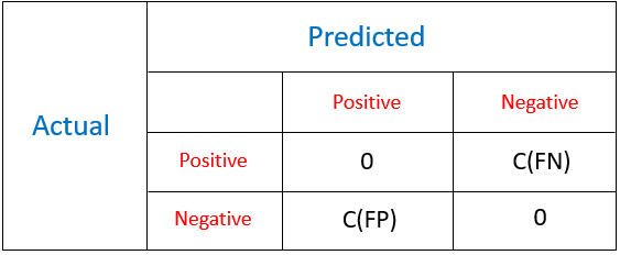
cost matrix cost selection algorithmCost Matrix

The goal of this method is to choose a classifier with lowest total cost.

Total Cost = C(FN)xFN + C(FP)xFP

where,

  1. FN is the number of positive observations wrongly predicted
  2. FP is the number of negative examples wrongly predicted
  3. C(FN) and C(FP) corresponds to the costs associated with False Negative and False Positive respectively. Remember, C(FN) > C(FP).

There are other advanced methods as well for balancing imbalanced data sets. These are Cluster based sampling, adaptive synthetic sampling, border line SMOTE, SMOTEboost, DataBoost – IM, kernel based methods and many more. The basic working on these algorithm is almost similar as explained above. There are more intuitive methods which you can try for improved predictions:

  1. Using clustering, divide the majority class into K distinct cluster. There should be no overlap of observations among these clusters. Train each of these cluster with all observations from minority class. Finally, average your final prediction.
  2. Collect more data. Aim for more data having higher proportion of minority class. Otherwise, adding more data will not improve the proportion of class imbalance.


Which performance metrics to use to evaluate accuracy ?

Choosing a performance metric is a critical aspect of working with imbalanced data. Most classification algorithms calculate accuracy based on the percentage of observations correctly classified. With imbalanced data, the results are high deceiving since minority classes hold minimum effect on overall accuracy.
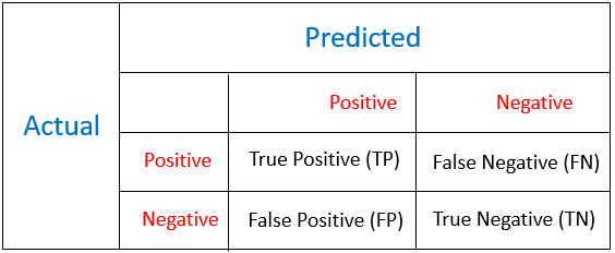
confusion matrix imbalanced classification metricConfusion Matrix

The difference between confusion matrix and cost matrix is that, cost matrix provides information only about the misclassification cost, whereas confusion matrix describes the entire set of possibilities using TP, TN, FP, FN. In a cost matrix, the diagonal elements are zero. The most frequently used metrics are Accuracy & Error Rate.

Accuracy: (TP + TN)/(TP+TN+FP+FN)

Error Rate = 1 - Accuracy = (FP+FN)/(TP+TN+FP+FN)

As mentioned above, these metrics may provide deceiving results and are highly sensitive to changes in data. Further, various metrics can be derived from confusion matrix. The resulting metrics provide a better measure to calculate accuracy while working on a imbalanced data set:

Precision: It is a measure of correctness achieved in positive prediction i.e. of observations labeled as positive, how many are actually labeled positive.

Precision = TP / (TP + FP)

Recall: It is a measure of actual observations which are labeled (predicted) correctly i.e. how many observations of positive class are labeled correctly. It is also known as ‘Sensitivity’.

Recall = TP / (TP + FN)

F measure: It combines precision and recall as a measure of effectiveness of classification in terms of ratio of weighted importance on either recall or precision as determined by β coefficient.

F measure = ((1 + β)² × Recall × Precision) / ( β² × Recall + Precision )

β is usually taken as 1.

Though, these methods are better than accuracy and error metric, but still ineffective in answering the important questions on classification. For example: precision does not tell us about negative prediction accuracy. Recall is more interesting in knowing actual positives. This suggest, we can still have a better metric to cater to our accuracy needs.

Fortunately, we have a ROC (Receiver Operating Characteristics) curve to measure the accuracy of a classification prediction. It’s the most widely used evaluation metric. ROC Curve is formed by plotting TP rate (Sensitivity) and FP rate (Specificity).

Specificity = TN / (TN + FP)

Any point on ROC graph, corresponds to the performance of a single classifier on a given distribution. It is useful because if provides a visual representation of benefits (TP) and costs (FP) of a classification data. The larger the area under ROC curve, higher will be the accuracy.

There may be situations when ROC fails to deliver trustworthy performance. It has few shortcomings such as.

  1. It may provide overly optimistic performance results of highly skewed data.
  2. It does not provide confidence interval on classifier’s performance
  3. It fails to infer the significance of different classifier performance.

As alternative methods, we can use other visual representation metrics include PR curve, cost curves as well. Specifically, cost curves are known to possess the ability to describe a classifier’s performance over varying misclassification costs and class distributions in a visual format. In more than 90% instances, ROC curve is known to perform quite well.


Imbalanced Classification in R

Till here, we’ve learnt about some essential theoretical aspects of imbalanced classification. It’s time to learn to implement these techniques practically.  In R, packages such as ROSE and DMwR helps us to perform sampling strategies quickly. We’ll work on a problem of binary classification.

ROSE (Random Over Sampling Examples) package helps us to generate artificial data based on sampling methods and smoothed bootstrap approach. This package has well defined accuracy functions to do the tasks quickly.

Let’s get started

#set path
> path <- "C:/Users/manish/desktop/Data/March 2016"

#set working directory
> setwd(path)

#install packages
> install.packages("ROSE")
> library(ROSE)

The package ROSE comes with an inbuilt imbalanced data set named as hacide. It comprises of two files: hacide.train and hacide.test. Let’s load it in R environment:

> data(hacide)
> str(hacide.train)
'data.frame': 1000 obs. of 3 variables:
$ cls: Factor w/ 2 levels "0","1": 1 1 1 1 1 1 1 1 1 1 ...
$ x1 : num 0.2008 0.0166 0.2287 0.1264 0.6008 ...
$ x2 : num 0.678 1.5766 -0.5595 -0.0938 -0.2984 ...

As you can see, the data set contains 3 variable of 1000 observations. cls is the response variable. x1 and x2 are dependent variables. Let’s check the severity of imbalance in this data set:

#check table
table(hacide.train$cls)
  0     1
980    20

#check classes distribution
prop.table(table(hacide.train$cls))
  0      1  
0.98   0.02

As we see, this data set contains only 2% of positive cases and 98% of negative cases. This is a severely imbalanced data set. So, how badly can this affect our prediction accuracy ? Let’s build a model on this data. I’ll be using decision tree algorithm for modeling purpose.

> library(rpart)
> treeimb <- rpart(cls ~ ., data = hacide.train)
> pred.treeimb <- predict(treeimb, newdata = hacide.test)

Let’s check the accuracy of this prediction. To check accuracy, ROSE package has a function names accuracy.meas, it computes important metrics such as precision, recall & F measure.

> accuracy.meas(hacide.test$cls, pred.treeimb[,2])
   Call:
   accuracy.meas(response = hacide.test$cls, predicted = pred.treeimb[, 2])
   Examples are labelled as positive when predicted is greater than 0.5 

   precision: 1.000
   recall: 0.200
   F: 0.167

These metrics provide an interesting interpretation. With threshold value as 0.5, Precision = 1 says there are no false positives. Recall = 0.20 is very much low and indicates that we have higher number of false negatives. Threshold values can be altered also. F = 0.167 is also low and suggests weak accuracy of this model.

We’ll check the final accuracy of this model using ROC curve. This will give us a clear picture, if this model is worth. Using the function roc.curve available in this package:

> roc.curve(hacide.test$cls, pred.treeimb[,2], plotit = F)
Area under the curve (AUC): 0.600

AUC = 0.60 is a terribly low score. Therefore, it is necessary to balanced data before applying a machine learning algorithm. In this case, the algorithm gets biased toward the majority class and fails to map minority class.

We’ll use the sampling techniques and try to improve this prediction accuracy. This package provides a function named ovun.sample which enables oversampling, undersampling in one go.

Let’s start with oversampling and balance the data.

#over sampling
> data_balanced_over <- ovun.sample(cls ~ ., data = hacide.train, method = "over",N = 1960)$data
> table(data_balanced_over$cls)
0    1
980 980

In the code above, method over instructs the algorithm to perform over sampling. N refers to number of observations in the resulting balanced set. In this case, originally we had 980 negative observations. So, I instructed this line of code to over sample minority class until it reaches 980 and the total data set comprises of 1960 samples.

Similarly, we can perform undersampling as well. Remember, undersampling is done without replacement.

> data_balanced_under <- ovun.sample(cls ~ ., data = hacide.train, method = "under", N = 40, seed = 1)$data
> table(data_balanced_under$cls)
0    1
20  20

Now the data set is balanced. But, you see that we’ve lost significant information from the sample. Let’s do both undersampling and oversampling on this imbalanced data. This can be achieved using method = “both“. In this case, the minority class is oversampled with replacement and majority class is undersampled without replacement.

> data_balanced_both <- ovun.sample(cls ~ ., data = hacide.train, method = "both", p=0.5,                             N=1000, seed = 1)$data
> table(data_balanced_both$cls)
0    1
520 480

p refers to the probability of positive class in newly generated sample.

The data generated from oversampling have expected amount of repeated observations. Data generated from undersampling is deprived of important information from the original data. This leads to inaccuracies in the resulting performance. To encounter these issues, ROSE helps us to generate data synthetically as well. The data generated using ROSE is considered to provide better estimate of original data.

> data.rose <- ROSE(cls ~ ., data = hacide.train, seed = 1)$data
> table(data.rose$cls)
0    1
520 480

This generated data has size equal to the original data set (1000 observations). Now, we’ve balanced data sets using 4 techniques. Let’s compute the model using each data and evaluate its accuracy.

#build decision tree models
> tree.rose <- rpart(cls ~ ., data = data.rose)
> tree.over <- rpart(cls ~ ., data = data_balanced_over)
> tree.under <- rpart(cls ~ ., data = data_balanced_under)
> tree.both <- rpart(cls ~ ., data = data_balanced_both)

#make predictions on unseen data
> pred.tree.rose <- predict(tree.rose, newdata = hacide.test)
> pred.tree.over <- predict(tree.over, newdata = hacide.test)
> pred.tree.under <- predict(tree.under, newdata = hacide.test)
> pred.tree.both <- predict(tree.both, newdata = hacide.test)

It’s time to evaluate the accuracy of respective predictions. Using inbuilt function roc.curve allows us to capture roc metric.

#AUC ROSE
> roc.curve(hacide.test$cls, pred.tree.rose[,2])
Area under the curve (AUC): 0.989

#AUC Oversampling
roc.curve(hacide.test$cls, pred.tree.over[,2])
Area under the curve (AUC): 0.798

#AUC Undersampling
roc.curve(hacide.test$cls, pred.tree.under[,2])
Area under the curve (AUC): 0.867

#AUC Both
roc.curve(hacide.test$cls, pred.tree.both[,2])
Area under the curve (AUC): 0.798

Here is the resultant ROC curve where:

  • Black color represents ROSE curve
  • Red color represents oversampling curve
  • Green color represents undersampling curve
  • Blue color represents both sampling curve

ROC curve

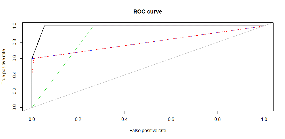
Hence, we get the highest accuracy from data obtained using ROSE algorithm. We see that the data generated using synthetic methods result in high accuracy as compared to sampling methods. This technique combined with a more robust algorithm (random forest, boosting) can lead to exceptionally high accuracy.

This package also provide us methods to check the model accuracy using holdout and bagging method. This helps us to ensure that our resultant predictions doesn’t suffer from high variance.

> ROSE.holdout <- ROSE.eval(cls ~ ., data = hacide.train, learner = rpart, method.assess = "holdout", extr.pred = function(obj)obj[,2], seed = 1)
> ROSE.holdout

Call:
ROSE.eval(formula = cls ~ ., data = hacide.train, learner = rpart,
extr.pred = function(obj) obj[, 2], method.assess = "holdout",
seed = 1)

Holdout estimate of auc: 0.985

We see that our accuracy retains at ~ 0.98 and shows that our predictions aren’t suffering from high variance. Similarly, you can use bootstrapping by setting method.assess to “BOOT”. The parameter extr.pred is a function which extracts the column of probabilities belonging to positive class.


End Notes

When faced with imbalanced data set, one might need to experiment with these methods to get the best suited sampling technique. In our case, we found that synthetic sampling technique outperformed the traditional oversampling and undersampling method. For better results, you can use advanced sampling methods which includes synthetic sampling with boosting methods.

In this article, I’ve discussed the important things one should know to deal with imbalanced data sets. For R users, dealing with such situations isn’t difficult since we are blessed with some powerful and awesome packages.

Did you find this article helpful ? Have you used these methods before? Do share your experience / suggestions in the comments section below.


Posted by uniqueone
,
http://machinelearningmastery.com/tactics-to-combat-imbalanced-classes-in-your-machine-learning-dataset/


8 Tactics to Combat Imbalanced Classes in Your Machine Learning Dataset

Has this happened to you?

You are working on your dataset. You create a classification model and get 90% accuracy immediately. “Fantastic” you think. You dive a little deeper and discover that 90% of the data belongs to one class. Damn!

This is an example of an imbalanced dataset and the frustrating results it can cause.

In this post you will discover the tactics that you can use to deliver great results on machine learning datasets with imbalanced data.

Class Imbalance

Find some balance in your machine learning.
Photo by MichaEli, some rights reserved.

Coming To Grips With Imbalanced Data

I get emails about class imbalance all the time, for example:

I have a binary classification problem and one class is present with 60:1 ratio in my training set. I used the logistic regression and the result seems to just ignores one class.

And this:

I am working on a classification model. In my dataset I have three different labels to be classified, let them be A, B and C. But in the training dataset I have A dataset with 70% volume, B with 25% and C with 5%. Most of time my results are overfit to A. Can you please suggest how can I solve this problem?

I write long lists of techniques to try and think about the best ways to get past this problem. I finally took the advice of one of my students:

Perhaps one of your upcoming blog posts could address the problem of training a model to perform against highly imbalanced data, and outline some techniques and expectations.

Frustration!

Imbalanced data can cause you a lot of frustration.

You feel very frustrated when you discovered that your data has imbalanced classes and that all of the great results you thought you were getting turn out to be a lie.

The next wave of frustration hits when the books, articles and blog posts don’t seem to give you good advice about handling the imbalance in your data.

Relax, there are many options and we’re going to go through them all. It is possible, you can build predictive models for imbalanced data.

What is Imbalanced Data?

Imbalanced data typically refers to a problem with classification problems where the classes are not represented equally.

For example, you may have a 2-class (binary) classification problem with 100 instances (rows). A total of 80 instances are labeled with Class-1 and the remaining 20 instances are labeled with Class-2.

This is an imbalanced dataset and the ratio of Class-1 to Class-2 instances is 80:20 or more concisely 4:1.

You can have a class imbalance problem on two-class classification problems as well as multi-class classification problems. Most techniques can be used on either.

The remaining discussions will assume a two-class classification problem because it is easier to think about and describe.

Imbalance is Common

Most classification data sets do not have exactly equal number of instances in each class, but a small difference often does not matter.

There are problems where a class imbalance is not just common, it is expected. For example, in datasets like those that characterize fraudulent transactions are imbalanced. The vast majority of the transactions will be in the “Not-Fraud” class and a very small minority will be in the “Fraud” class.

Another example is customer churn datasets, where the vast majority of customers stay with the service (the “No-Churn” class) and a small minority cancel their subscription (the “Churn” class).

When there is a modest class imbalance like 4:1 in the example above it can cause problems.

Accuracy Paradox

The accuracy paradox is the name for the exact situation in the introduction to this post.

It is the case where your accuracy measures tell the story that you have excellent accuracy (such as 90%), but the accuracy is only reflecting the underlying class distribution.

It is very common, because classification accuracy is often the first measure we use when evaluating models on our classification problems.

Put it All On Red!

What is going on in our models when we train on an imbalanced dataset?

As you might have guessed, the reason we get 90% accuracy on an imbalanced data (with 90% of the instances in Class-1) is because our models look at the data and cleverly decide that the best thing to do is to always predict “Class-1” and achieve high accuracy.

This is best seen when using a simple rule based algorithm. If you print out the rule in the final model you will see that it is very likely predicting one class regardless of the data it is asked to predict.

8 Tactics To Combat Imbalanced Training Data

We now understand what class imbalance is and why it provides misleading classification accuracy.

So what are our options?

1) Can You Collect More Data?

You might think it’s silly, but collecting more data is almost always overlooked.

Can you collect more data? Take a second and think about whether you are able to gather more data on your problem.

A larger dataset might expose a different and perhaps more balanced perspective on the classes.

More examples of minor classes may be useful later when we look at resampling your dataset.

2) Try Changing Your Performance Metric

Accuracy is not the metric to use when working with an imbalanced dataset. We have seen that it is misleading.

There are metrics that have been designed to tell you a more truthful story when working with imbalanced classes.

I give more advice on selecting different performance measures in my post “Classification Accuracy is Not Enough: More Performance Measures You Can Use“.

In that post I look at an imbalanced dataset that characterizes the recurrence of breast cancer in patients.

From that post, I recommend looking at the following performance measures that can give more insight into the accuracy of the model than traditional classification accuracy:

  • Confusion Matrix: A breakdown of predictions into a table showing correct predictions (the diagonal) and the types of incorrect predictions made (what classes incorrect predictions were assigned).
  • Precision: A measure of a classifiers exactness.
  • Recall: A measure of a classifiers completeness
  • F1 Score (or F-score): A weighted average of precision and recall.

I would also advice you to take a look at the following:

  • Kappa (or Cohen’s kappa): Classification accuracy normalized by the imbalance of the classes in the data.
  • ROC Curves: Like precision and recall, accuracy is divided into sensitivity and specificity and models can be chosen based on the balance thresholds of these values.

You can learn a lot more about using ROC Curves to compare classification accuracy in our post “Assessing and Comparing Classifier Performance with ROC Curves“.

Still not sure? Start with kappa, it will give you a better idea of what is going on than classification accuracy.

3) Try Resampling Your Dataset

You can change the dataset that you use to build your predictive model to have more balanced data.

This change is called sampling your dataset and there are two main methods that you can use to even-up the classes:

  1. You can add copies of instances from the under-represented class called over-sampling (or more formally sampling with replacement), or
  2. You can delete instances from the over-represented class, called under-sampling.

These approaches are often very easy to implement and fast to run. They are an excellent starting point.

In fact, I would advise you to always try both approaches on all of your imbalanced datasets, just to see if it gives you a boost in your preferred accuracy measures.

You can learn a little more in the the Wikipedia article titled “Oversampling and undersampling in data analysis“.

Some Rules of Thumb

  • Consider testing under-sampling when you have an a lot data (tens- or hundreds of thousands of instances or more)
  • Consider testing over-sampling when you don’t have a lot of data (tens of thousands of records or less)
  • Consider testing random and non-random (e.g. stratified) sampling schemes.
  • Consider testing different resampled ratios (e.g. you don’t have to target a 1:1 ratio in a binary classification problem, try other ratios)

4) Try Generate Synthetic Samples

A simple way to generate synthetic samples is to randomly sample the attributes from instances in the minority class.

You could sample them empirically within your dataset or you could use a method like Naive Bayes that can sample each attribute independently when run in reverse. You will have more and different data, but the non-linear relationships between the attributes may not be preserved.

There are systematic algorithms that you can use to generate synthetic samples. The most popular of such algorithms is called SMOTE or the Synthetic Minority Over-sampling Technique.

As its name suggests, SMOTE is an oversampling method. It works by creating synthetic samples from the minor class instead of creating copies. The algorithm selects two or more similar instances (using a distance measure) and perturbing an instance one attribute at a time by a random amount within the difference to the neighboring instances.

Learn more about SMOTE, see the original 2002 paper titled “SMOTE: Synthetic Minority Over-sampling Technique“.

There are a number of implementations of the SMOTE algorithm, for example:

  • In Python, take a look at the “UnbalancedDataset” module. It provides a number of implementations of SMOTE as well as various other resampling techniques that you could try.
  • In R, the DMwR package provides an implementation of SMOTE.
  • In Weka, you can use the SMOTE supervised filter.

5) Try Different Algorithms

As always, I strongly advice you to not use your favorite algorithm on every problem. You should at least be spot-checking a variety of different types of algorithms on a given problem.

For more on spot-checking algorithms, see my post “Why you should be Spot-Checking Algorithms on your Machine Learning Problems”.

That being said, decision trees often perform well on imbalanced datasets. The splitting rules that look at the class variable used in the creation of the trees, can force both classes to be addressed.

If in doubt, try a few popular decision tree algorithms like C4.5, C5.0, CART, and Random Forest.

For some example R code using decision trees, see my post titled “Non-Linear Classification in R with Decision Trees“.

For an example of using CART in Python and scikit-learn, see my post titled “Get Your Hands Dirty With Scikit-Learn Now“.

6) Try Penalized Models

You can use the same algorithms but give them a different perspective on the problem.

Penalized classification imposes an additional cost on the model for making classification mistakes on the minority class during training. These penalties can bias the model to pay more attention to the minority class.

Often the handling of class penalties or weights are specialized to the learning algorithm. There are penalized versions of algorithms such as penalized-SVM and penalized-LDA.

It is also possible to have generic frameworks for penalized models. For example, Weka has a CostSensitiveClassifier that can wrap any classifier and apply a custom penalty matrix for miss classification.

Using penalization is desirable if you are locked into a specific algorithm and are unable to resample or you’re getting poor results. It provides yet another way to “balance” the classes. Setting up the penalty matrix can be complex. You will very likely have to try a variety of penalty schemes and see what works best for your problem.

7) Try a Different Perspective

There are fields of study dedicated to imbalanced datasets. They have their own algorithms, measures and terminology.

Taking a look and thinking about your problem from these perspectives can sometimes shame loose some ideas.

Two you might like to consider are anomaly detection and change detection.

Anomaly detection is the detection of rare events. This might be a machine malfunction indicated through its vibrations or a malicious activity by a program indicated by it’s sequence of system calls. The events are rare and when compared to normal operation.

This shift in thinking considers the minor class as the outliers class which might help you think of new ways to separate and classify samples.

Change detection is similar to anomaly detection except rather than looking for an anomaly it is looking for a change or difference. This might be a change in behavior of a user as observed by usage patterns or bank transactions.

Both of these shifts take a more real-time stance to the classification problem that might give you some new ways of thinking about your problem and maybe some more techniques to try.

8) Try Getting Creative

Really climb inside your problem and think about how to break it down into smaller problems that are more tractable.

For inspiration, take a look at the very creative answers on Quora in response to the question “In classification, how do you handle an unbalanced training set?

For example:

Decompose your larger class into smaller number of other classes…

…use a One Class Classifier… (e.g. treat like outlier detection)

…resampling the unbalanced training set into not one balanced set, but several. Running an ensemble of classifiers on these sets could produce a much better result than one classifier alone

These are just a few of some interesting and creative ideas you could try.

For more ideas, check out these comments on the reddit post “Classification when 80% of my training set is of one class“.

Pick a Method and Take Action

You do not need to be an algorithm wizard or a statistician to build accurate and reliable models from imbalanced datasets.

We have covered a number of techniques that you can use to model an imbalanced dataset.

Hopefully there are one or two that you can take off the shelf and apply immediately, for example changing your accuracy metric and resampling your dataset. Both are fast and will have an impact straight away.

Which method are you going to try?

A Final Word, Start Small

Remember that we cannot know which approach is going to best serve you and the dataset you are working on.

You can use some expert heuristics to pick this method or that, but in the end, the best advice I can give you is to “become the scientist” and empirically test each method and select the one that gives you the best results.

Start small and build upon what you learn.

Want More? Further Reading…

There are resources on class imbalance if you know where to look, but they are few and far between.

I’ve looked and the following are what I think are the cream of the crop. If you’d like to dive deeper into some of the academic literature on dealing with class imbalance, check out some of the links below.

Books

Papers

Did you find this post useful? Still have questions?

Leave a comment and let me know about your problem and any questions you still have about handling imbalanced classes.

Posted by uniqueone
,

https://www.quora.com/In-classification-how-do-you-handle-an-unbalanced-training-set


In classification, how do you handle an unbalanced training set?

In some cases, you have a lot more examples of one class than of the others. How do you tackle this problem? What are some gotchas to be aware of in this situation?
30 Answers
Sergey Feldman
Sergey Feldman, machine learning PhD & consultant @ www.data-cowboys.com

the ones listed above/below are great! here are a few more:

1) let's say you have L more times of the abundant class than rare class. for stochastic gradient descent, take L separate steps each time you encounter training data from the rare class.

2) divide the more abundant class into L distinct clusters. then train L predictors, where each predictor is trained on only one of the distinct clusters, but on all of the data from the rare class. to be clear, the data from the rare class is used in the training of all L predictors. finally, use model averaging for the L learned predictors as your final predictor.

3) this is similar to Kripa's number (2), but a little different.
let N be number of samples in the rare class. cluster the abundant
class into N clusters (agglomerative clustering may be best here), and use the resulting cluster mediods as the training data for the abundant class. to be clear, you throw out the original training data from the abundant class, and use the mediods instead. voila, now your classes are balanced!

4) whatever method you use will help in some ways, but hurt in others. to mitigate that, you could train a separate model using all of the methods listed on this page, and then perform model averaging over all of them!

5) A recent ICML paper (similar to Kripa's (1)) shows that adding data that are "corrupt[ed] training examples with noise from known distributions" can actually improve performance. The paper isn't totally relevant to the problem of unbalanced classes because they add the data implicitly with math (that is, the dataset size remains unchanged). But I think the table of corrupting distributions in the paper is useful if you want to implement your own surrogate data code.

More details than you need: imho, the most interesting of the corrupting distributions is the blankout distribution, where you just zero out a random subset of features. Why is it interesting? Because you are helping your classifier be sturdier/hardier by giving it variations of your data that have essentially missing features. So it has to learn to classify correctly even in adverse conditions.

A related idea is dropout in neural networks, where random hidden units are removed (zeroed-out) during training. This forces the NN to, again, be hardier than it would be otherwise. See here for a recent treatment: http://www.stanford.edu/~sidaw/c...

Here’s a nice package that does a lot of this stuff and is compatible with the scikit-learn API: scikit-learn-contrib/imbalanced-learn

Roar Nybø
Roar Nybø, Using ML for diagnostics in offshore drilling
The data set example has a strong class imbalance, which can mislead some classification algorithms. In particular, some will always output '0' since that is correct in 99.97% of cases. The easiest remedy is to train on just 300 examples from each class.
However, you also have to consider the following:
  1. Are the almost 1 million examples labeled '0' similar enough to be captured by one class, or is it simpler from an ML point of view, to work with many sub-classes?
  2. Are the 300 examples labeled '1' representative of the class, or are there parts of the parameter space that is simply not covered, because we have too few examples?
  3. What is the misclassification rate? If in class '0', only one in every ten thousandth example got misclassified, those misclassifications would still make up half of the examples in class '1'.

One situation where this occurs is intrusion detection in computer networks. Almost all network traffic is legitimate, with viruses and hacking attempts making up only a tiny amount, so this will yield a data set with a strong class imbalance. We also lack a representative collection of intrusion attempts, because new methods are developed all the time. The intrusion class is an open class.
When classes not seen in the training set may appear in later use, the problem is referred to as open set classification [1].

Methods to deal with issue 2 includes anomaly detection and one-class learning. Here the goal is to draw a line around a well-documented class and classify cases as simply belonging or not belonging to that class. In the
example above you'd flag as intrusion anything not similar to normal traffic. In [2] issue 1 and 2 is attacked simultaneously, by using an ensemble of one-class classifiers. (Actually the same strategy as Charles H Martin is proposing here.)

Issue 3 is a hard one, but ensembles of classifiers can be of some use in this regard as well. If none of the one-class classifiers fire on an example, this can be taken as an indication that the example is hard to classify. This is an improvement over binary classifiers, which by virtue of the decision boundary will always try to classify every example.

[1] GORI, M. & SCARSELLI, F. (1998) Are multilayer perceptrons adequate for pattern recognition and verification? Ieee Transactions on Pattern Analysis and
Machine Intelligence, 20, 1121-1132
[2] GIACINTO, G., PERDISCI, R., DEL RIO, M. & ROLI, F. (2008) Intrusion detection in computer networks by a modular ensemble of one-class classifiers.
Information Fusion, 9, 69-82.
Abhishek Ghose
Abhishek Ghose, Data Scientist @[24]7
This is a very practical problem and here are some ways to get around this:
  1. Random undersampling of the majority class
  2. Random oversampling of the minority class
  3. Random undersampling leads to potential loss of information - since a lot of data instances are just 'thrown away'. You can perform informed undersampling by finding out the distribution of data first and selectively pick points to be thrown away
  4. You can oversample with synthetically generated data points that are not too different from the minority class data points you actually have - SMOTE  is a popular technique.
  5. Use a cost-sensitive classifier. For example, in certain kinds of decision trees (ex C5.0: An Informal Tutorial) you can explicitly mention that misclassifying a data instance from the minority class as the majority class is much more expensive than the other kind of misclassification. libsvm, the popular SVM package, allows this using the "wx" flags.

The above list is not exhaustive. This paper provides a good survey: http://www.ele.uri.edu/faculty/h...

Make sure that you are using a scoring mechanism that deals with imbalance. For ex, if your data 97% -ve and 3% +ve, using accuracy as a performance metric I can easily score 97% by classifying all points as -ve. So, accuracy is not a good metric here; something like F1-score is more suitable.
Ian Vala
Ian Vala, Senior Data Scientist working in Silicon Valley. Harvard grad.

Haha you know whats funny? You get 90% accuracy for your model and you are like “awesome!” until you find out, well %90 of the data was all on one class lol

This is actually a very good interview question and what you are referring to is called “imbalanced data”.It is a very common problem when you get a real dataset. For example you get cancer patient data. They tell you go predict if the person has cancer or not. Great! Making the world a better place, and making 6 figure salary! You are excited and get the dataset, it’s 98% no cancer and 2% cancer.

Crap…

Lo and behold, thankfully there are some solutions for this:

  1. Resample differently. Over-sample from your minority class and under-sample from your majority class, so you get a more balanced dataset.
  2. Try different metrics other than correct vs wrong prediction. Try Confusion Matrix or ROC curve. Accuracy is divided into sensitivity and specificity and models can be chosen based on the balance thresholds of the values.
  3. Use Penalized Models. Like penalized-SVM and penalized-LDA. They put additional cost on the model for making classification mistakes on the minority class during training. These penalties can bias the model towards paying attention to minority class.
  4. Try Anomaly Detection techniques and models often used there. Although that would probably be necessary if your data was even more Imbalanced.

Still not satisfied? Here’s the book on this: Imbalanced Learning: Foundations, Algorithms, and Applications: Haibo He, Yunqian Ma: 9781118074626: Amazon.com: Books

Kripa Chettiar
Kripa Chettiar, NLP and ML practitioner; Personalization @ Amazon - Music Recommendations
You could do either of the following:

  1. Generate synthetic data using SMOTE or SMOTEBoost.[http://wiki.pentaho.com/display/... ]. This should give you good results in more cases.
  2. Decompose your larger class into smaller number of other classes. This is tricky and totally dependent on the kind of data you have. For something like 30 instances of A vs 4000 instances of B, you would decompose the 4000 instances of B into 1000 instances of B1 and 3000 instances of unknown. Effectively you are reducing the difference in number of instances between A and B1.
  3. A medly of 1 and 2 could also work.
  4. In the worst case use a One Class Classifier. What you are doing here is that you are considering the smaller class an outlier and confidently learn the decision boundary for ONLY the larger class. Weka provides a one-class classifier library. [http://webcache.googleuserconten...
5. Get more data!
Dayvid Victor
Dayvid Victor, Machine Learning Researcher | PhD candidate in Computer Science | Data Scientist

There are a few notes and suggestions:

  1. Regular classification rate (classification accuracy) isn't a good metric, because if you correctly classify only the instances of the majority class
    (class with many samples), this metric still gives you a high rate.
    The Area Under the ROC Curve (AUC) is a good metric for evaluation of classifiers in such datasets.
  2. You can increase the number of minority class samples by:
    1. Resampling: bootstrapping samples of the minority class.
    2. Oversampling: generate new samples of the minority class, for this, I'd recommend to use SMOTE, SPIDER or any variant. You can also use Prototype Generation (PG) in order to generate new samples of the minority class - there are specific PG techniques for imbalanced datasets such as ASGP and EASGP.
  3. You can reduce the number of majority class samples by:
    1. Random Undersampling.
    2. Prototype Selection (PS) to reduce imbalance level, such as One-Sided Selection (OSS). Or, you can use Tomek Links, Edited-Nearest Neighbors (ENN) and other but only remove the majority class outliers.
  4. In your K-Fold validation, try to use the same proportion between the classes. If the number of instances of the minority class is too low, you can reduce the number of K, until there are enough.
  5. Use Multiple Classifier Systems (MCS):
    1. Using Ensemble Learning has been proposed as an interesting solution to learn from imbalanced data.

Also, be careful with the techniques/algorithms you will use. In prototype generation, for example, there are techniques that have a high performance on regular datasets, but if you use them with unbalanced datasets, they will misclassify most (or all) instances of the minority class.

In cases like that, search for a similar algorithm, adapted to handle unbalanced datasets, or adapt it yourself. If you get good results, you can even publish it (I've done that).

Yevgeny Popkov
Yevgeny Popkov, Data Scientist @ CQuotient
These two alternative approaches are typically used:
1) Quick&dirty approach: balance the data set by either under-sampling the majority class(es) or over-sampling the minority class(es).
2) A preferred approach: use cost-sensitive learning by applying class-specific weights in your loss function (smaller weights for the majority class cases and larger weights for the minority class cases). For starters, the weights can be set to be inversely proportional to the fraction of cases of the corresponding class.  In case of binary classification the weight of one of the classes can be tuned using resampling to squeeze even more predictive power out of the model.
Qingbin Li
Qingbin Li, Data Scientist @ ServiceNow | Machine Learning Enthusiast

When dealing with imbalanced classification problem, I would consider the following aspects :

  1. Whether more data could be collected or not. Sometime the dataset is imbalanced because we don’t collect enough data.
  2. Utilize techniques to balance the data. We can consider downsampling the majority class or upsampling the minority class or generating synthetic data, etc. The main goal is to convert the imbalanced classification problem into a balanced classification problem so the regular classification algorithms can be used.
  3. Choose the algorithm that is insensitive to imbalance data, like cost-sensitive learning. The basic idea is to adjust the cost of various classes.
  4. Use the correct performance metric, like AUC, f-score, Confusion Matrix, etc. It’s quite important to choose the right metric to evaluate your model performance.
Charles H Martin
Charles H Martin, Calculation Consulting; we predict things
I woud just try the simplest ting possible... train a bunch of binary SVMs with equal balance of positive and random negative samples and majority vote as the label.

I have this problem all the time in industry...sometimes something just bone head simple works quite well

---

Additionally...ask yourself "why would a simple SVM fail (using class weights)?" After all, the SVM only learns from data on the margin, so, in theory, the mis-balanced classes should not matter.  There are two reasons:

1.  You are using mean squared error to evaluate the accuracy during cross validation.  Another metric may suit your problem better

2.  The data is non-separable without adding some slack, andyou can not adjust more than a single  regularization parameter (and a few kernel parameters), and therefore you can can not control the slack at the margin...where the data is non-seperable.

 By selecting N random sets rather than class weights, the hope is you can adjust the slack variables on each set.  Vapnik has developed a 'similar' approach, which he calls "Master Learning" (although here the Master knowledge is information add by adjusting the] slack variables 

of course, if you find the regularization and kernel parameters are the same for every random sample, you may not have gained anything
Muktabh Mayank
Muktabh Mayank, Data Scientist,CoFounder @ ParallelDots, BITSian for life, love new technology trends
Here is a recent paper which addresses the same problem. It uses a method similar to SVM.
I am working on an implementation, will open source it soon. Page on hal.inria.fr

There is a nice method to cope with unbalanced data set with a theoretical justification.
The method is based of the boosting algorithm Robert E. Schapire presented at "The strength of weak learnability" (Machine Learning, 5(2):197–227, 1990. http://rob.schapire.net/papers/s... ).

In this paper Schapire presented a boosting algorithm based upon combining triplets of 3 weak learners recursively. By the way, this was the first boosting algorithm.

We can use the first step of the algorithm (even without the recursion) to cope with the lack of balance.

The algorithm trains the first learner, L1, on the original data set.
The second learner, L2, is train on a set on which L1 has 50% chance to be correct (by sampling from the original distribution).
The third learner, L3, is trained on the cases on which L1 and L2 disagree.
As output, return the majority of the classifiers.
See the paper to see why it improves the classification.

Now for the application of the method of an imbalanced set.
Assume the concept is binary and the majority of the samples are classified as true.

Let L1 return always true.
L2, is being trained where L1 has 50% to be right. Since L1 is just true, L2 is being training on a balanced data set.
L3 is being trained when L1 and L2 disagree, hence, when L2 predicts false.
The ensemble predicts by majority, hence predicts false only when both L2 and L3 predict false.

I used this method in practice many times and it is very useful.

Kaushik Kasi
Kaushik Kasi, (Data Science && Bitcoin) Enthusiast
Here are some options
  • Replicate data points for the lagging class and add those to the training data (might increase bias)
  • Artificially generate more data points by manually tweaking features. This is sometimes done with with systems involving images, where an existing image can be distorted to create a new image. You run the risk of training the model based on (artificial) samples that aren't representative of the test samples that the model would encounter in the real world.
  • Treat the multi-class classifier as a binary classifier for the larger sample. Define the larger class as positive and the smaller class as a negative. This would train your model distinctly on what the larger class looks like, and theoretically classifier the smaller class as "negatives". Your performance will depend on how many features you have for your samples and how tolerant your model can be to overfitting.
Aayush
Aayush, Data Science Intern

I’d recommend three ways to solve the problem, each has (basically) been derived from Chapter 16: Remedies for Severe Class Imbalance of Applied Predictive Modeling by Max Kuhn and Kjell Johnson.

  1. Random Forests w/ SMOTE Boosting: Use a hybrid SMOTE that undersamples the majority class and generates synthetic samples for the minority class by adjustable percentages. Select these percentages depending on the distribution of your response variable in the training set. Feed this data to your RF model. Always cross-validate/perform gird-search to find the best parameter settings for your RFs.
  2. XGBoost w/ hyper-parameter optimisation: Again, cross-validate or perform gird-search to find the best parameter settings for the model. I found this post extremely useful in my case. Additionally, xgboost offers parameters to balance positive and negative weights using scale_pos_weight. See the parameter documentation for a complete list.
  3. Support Vector Machines w/ Cost Sensitive Training:
    - SVMs allow for some degree of mis-classification of data and then repeatedly optimizes a loss function to find the required “best fit” model.
    - It controls the complexity using a cost function that increases the penalty if samples are on the incorrect side of the current class boundary.
    - For class imbalances, unequal costs for each class can adjust the parameters to increase or decrease the sensitivity of the model to particular classes.

I have used methods one and two and have been able to obtain an AUC of over 0.8 on the test data-set, and the data-set I was working on had very serious class imbalance with the minority class making up as little as 0.26% of the data-set.

Some important advice that I received and I’d like to give to anyone dealing with severely skewed classes is that:

  • Understand your data. Know what your requirements are and what type of classification matters more to you and which classification are you willing to trade-off.
  • Do not use % accuracy as a metric, use AUC, Sensitivity-Specificity and Cohen’s Kappa scores instead. The fundamental problem with using accuracy as a metric is that your model can simply classify everything into the majority class and give you a very high accuracy which is definitely one of the biggest “gotchas”, as mentioned in the question.
  • Run a lot of tests on multiple models. Intuition can take you a long way in data-science - if your gut tells you that an ensemble of classifiers will give you the best results, go ahead and try it.

On a closing note, I’d like to say here that XGBoost when tuned correctly has rarely ever disappointed anyone, but that shouldn’t stop you from experimenting!

Shehroz Khan
Shehroz Khan, ML Researcher, Postdoc @U of Toronto

To handle skewed data, you can employ different strategies, such as

  • Over sampling the minority class or under sampling the majority class
  • Cost sensitive classification
  • One-class Classification

You can read my detailed answer to a similar question here - Shehroz Khan's answer to I have an imbalanced dataset with two classes. Would it be considered OK if I oversample the minority class and also change the costs of misclassification on the training set to create the model?

C.V. Krishnakumar
C.V. Krishnakumar, studied Computer Science at Stanford University (2010)
Here is my opinion on this. Please take it with a grain of salt, since the answer might differ with different applications.
  • Gotcha #1: Do not use accuracy alone as a metric. That way, we would get 99% accuracy with everything classified as the majority class, which would not mean anything. Precision & Recall, with respect to each class might be a better one.
  • If you are more  interested in the classification of the  minority class, you can use a Cost sensitive classifier (http://weka.wikispaces.com/CostS...) through which you can state the cost of misclassification of the different classes. Eg. Misclassifying the minority might be considered to be costlier.
  • You might want to boost the number of minority class training examples by artificially creating new samples from the existing samples.
  • Simplest of all, you could also just resample the set, to have a proportional number of samples in both the classes, if that is an option.
Feng Qi (奇峰)
Feng Qi (奇峰), Software Engineer, Quora
1. assign higher weights to training data of rare classes
2. up-sampling rare class
3. sometimes highly imbalanced data can still give good training results. I think it makes sense for some metrics, for example, auc.

I found this blogpost to be helpful.

In short - use F1 scoring, and pick an algorithm that can handle unbalanced classes by weighting samples differently by class.

I did not find sub sampling very helpful because my rare class was only 3% of observations and that led to too little data for my algorithm to work with.

Yiyao Liu
Yiyao Liu, improving every day

In this article: Practical Guide to deal with Imbalanced Classification Problems in R, it mentioned four methods with some cases, which are clear and helpful.

  1. Undersampling
  2. Oversampling
  3. Synthetic Data Generation
  4. Cost Sensitive Learning
Adding to what Krishnakumar said and specifically the third point of generating artificial or synthetic samples of the minority class to maintain a balance, check out this paper on SMOTE(Synthetic Minority Oversampling TEchnique) - http://arxiv.org/pdf/1106.1813.pdf. It seems to be using a nearest neighbor approach to generate synthetic samples of the minority class. In all probability, there will be a lot of noise in the artificial samples generated.

I did have quite a bit of success in using this approach to classify credit card transactions as fraudulent.
If you are looking to use a Support Vector Machine for classification, you may consider using the Twin SVM which is suited to unbalanced datasets.
@Twin Support Vector Machines for Pattern Classification
The objective is two find two separating hyperplanes, each of which is closer to points of one class and far from points of the other. Predictions on test points are computed based on the distance from the two hyperplanes.
Todd Jamison
Todd Jamison, Imagery Scientist, develop machine learning algorithms for earth observation

In our software, we use an accuracy metric that balances the Producer’s and User’s accuracy and applies a larger penalty for higher levels of error. It can accommodate any number of classes, not just binary problems. Our accuracy function equation is:

where:

N = the number of classes,

Mn = the number of data points in each class,

Rn = the number of data points assigned to the class by the solution,

pni = the classification results for the ith training sample in class n, and

rni = the classification results for the ith training sample assigned to class n.

There are two items within the primary summation. The first item is related to the Producer’s Accuracy and the second is related to the User’s Accuracy. In this formula, we calculate the Producer’s and User’s error rates for each class instead of the accuracy rates by inverting the results values (i.e., (1-pni) and (1-rni) respectively). The error rates in the range 0 to 1 are root-mean-squared, in order to emphasize larger error rates. The error metric is then converted back to an accuracy metric by subtracting the result from 1. If you are using it as a cost function, you don’t do the final subtraction.

This metric should result in solutions that have a more balanced level of accuracy across classes and between Producer and User perspectives.

Nigel Legg
Nigel Legg, Discovering meaning in your data.
This is actually something I'm thinking about right now.  I have a data file of 49,000 records that need to be pushed through the classifier.  We have two classifications, Yes and No. From experience with a smaller data file, we will get >99% No, and <1% Yes, but the Yes classification is the important one. So I have manually classified 200 records, for the training set (gave 2xYes, 198xNo), and this is currently queued to be classified.
I'm assuming that this will give some odd results - there aren't enough examples of the 'Yes' classification.  I think a better training set would be a more balanced one, in spite of the inbalance in the test set.  Thus a better approach would be to hunt out the 'Yes' records to ensure that there are >50 classified in the training set.  The danger with this, however, is that you could end up classifying all the 'Yes' records by hand, leaving nothing for the classifier to do. ;-)
Alex Gilgur
Alex Gilgur, Data Scientist; IT Analyst; occasional lecturer at UCBerkeley's MIDS program.

I think you are referring to an imbalanced, rather than skewed, dataset. Regardless, it is a big problem in classification, because as you pointed out, data are rarely balanced. One way to solve it is, when training your classifier, to sample separately from the positive and the negative sets and combine them 9:1 when done: it's all about conditional probabilities.

Prem R. Adhikari
Prem R. Adhikari, Machine learning student and learner
Here you will find 8 Tactics to Combat Imbalanced Classes in Your Machine Learning Dataset - Machine Learning Mastery
I will like to add that ideas suggested in the link and by Abhishek Ghose, it is not the choice of classification algorithm but the classification metric that is important for imbanced datasets. AUC, F-measure, and logloss are often used in imbalanced datasets.
Ziyu Yao
Ziyu Yao, studied at Beijing University of Posts and Telecommunications
When I worked on social spam detection, I met the same problem. I think I can give some ideas:
1. For training step, you can perform under-sampling for unbalanced training dataset;
2. For testing step, some measurements can be  fair enough to evaluate your model. In my experience, AUC curve, Lift Chart and F-measure can be very helpful. You can try them.
Hope my advices can help you.
Have a look at down/up sampling methods and hybrid one like SMOTE

You can also play with the threshold (default=0.5) in order to reach a specific precision or specificity requirement, but it's more artificial.

NB: if your class is not well balanced don't choose the accuracy as your evaluation metric (ex: Y={0:90%, 1:10%} then for a the silly Y_hat=0 you get an accuracy of 90%) one could prefer the AUC (Area Under the Curve)
I would recommend using an error metric that is not sensitive to the imbalance between the classes. My personal favorite is AUC.

See What is the best out-of-sample accuracy test for a logistic regression and why? for more on this.
Quora User
Quora User, studied at Stanford University
I deal almost exclusively with this problem in the workplace.  Usually undersampling the 0 class (which I will assume, WLOG, is the larger one) is the right way to do this.
We encounter this scenario often in online advertising (specifically display advertising) where conversion rate is really low. I have experimented several methods but the method that gave me the best result was using binary classifier (logistic or SVM) with appropriate weight on negative and positive instances.  There are several tricks to compute these weights and they depend on profit and cost associated with positive and negative example respectively.

A good read on this topic is: Learning from Imbalanced Classes

Posted by uniqueone
,

머신 러닝(Machine Learning) - Class 67 : Semantic Segmentation – “Selective Search (part2)” : 네이버 블로그
http://blog.naver.com/laonple/220925179894
Posted by uniqueone
,

http://warmspringwinds.github.io/tensorflow/tf-slim/2017/01/23/fully-convolutional-networks-(fcns)-for-image-segmentation/


Fully Convolutional Networks (FCNs) for Image Segmentation

A post showing how to perform Image Segmentation using Fully Convolutional Networks that were trained on PASCAL VOC using our framework.


Introduction

In this post we want to present Our Image Segmentation library that is based on Tensorflow and TF-Slim library, share some insights and thoughts and demonstrate one application of Image Segmentation.

To be more precise, we trained FCN-32s, FCN-16s and FCN-8s models that were described in the paper “Fully Convolutional Networks for Semantic Segmentation” by Long et al. on PASCAL VOC Image Segmentation dataset and got similar accuracies compared to results that are demonstrated in the paper.

We provide all the training scripts and scripts to convert PASCAL VOC into easier-to-use .tfrecords file. Moreover, it is very easy to apply the same scripts to a custom dataset of your own.

Also, in the repository, you can find all the trained weights and scripts to benchmark the provided models against PASCAL VOC. All the FCN models were trained using VGG-16 network initialization that we took from TF-Slim library.

After that, we demonstrate how to create your own stickers for Telegram messaging app using our pretrained models, as a Qualitative Evaluation of our trained models. While the Quantitative Results are presented in the repository.

The blog post is created using jupyter notebook. After each chunk of a code you can see the result of its evaluation. You can also get the notebook file from here.

Training on PASCAL VOC

The models were trained on Augmented PASCAL VOC dataset which is mentioned in the paper by Long et al. The FCN-32s model was initialized from VGG-16 model and trained for one hundred thousand iterations. The FCN-16s was initialized with FCN-32s weights and also trained for one hundred thousand iterations. FCN-8s was trained in the same fashion with initialization from FCN-16s model.

The reason why the authors of the paper add skips is because the results produced by the FCN-32s architecture are too coarse and skips are added to lower layers of the VGG-16 network which were affected by smaller number of max-pooling layers of VGG-16 and, therefore, can give finer predictions while still taking into account more reliable higher level predictions.

During the training, we noticed that the cross entropy loss was decreasing, after we added skips that FCN-16s and FCN-8s models have. Also, during the training we randomly change the scale of the training image. Due to this fact, we had to normalize the cross entropy loss, because, otherwise, it was hard to understand if the loss is decreasing (we had different number of pixels on each iteration stage as a result of random scaling). Here you can see the cross entropy loss plot:

png

We trained with a batch size one and used Adam optimizer. It is important to state here, that although we trained with a batch size one, which might sound crazy – it actually means that after we do forward propagation for one image, we get predictions for each pixel. Then, we compute the pixel-wise cross-entropy. So, batch size one only means that we use one image per iteration, which consists of pixel-wise training samples.

Overall, we achieved comparable or better performance with the original paper. You can find our results in the repository.

Qualitative results

In order to show some results of Segmentation produced by aforementioned models, let’s apply the trained models to unseen images that contain some objects that represent one of PASCAL VOC classes. After we get segmentation masks, we create a countour for our segmentation masks, to create stickers and we save everything as a png file with alpha channel, to display only object and make background transparent.

%matplotlib inline

from __future__ import division

import os
import sys
import tensorflow as tf
import skimage.io as io
import numpy as np

sys.path.append("tf-image-segmentation/")
sys.path.append("/home/dpakhom1/workspace/my_models/slim/")

fcn_16s_checkpoint_path = \
 '/home/dpakhom1/tf_projects/segmentation/model_fcn8s_final.ckpt'

os.environ["CUDA_VISIBLE_DEVICES"] = '1'

slim = tf.contrib.slim

from tf_image_segmentation.models.fcn_8s import FCN_8s
from tf_image_segmentation.utils.inference import adapt_network_for_any_size_input
from tf_image_segmentation.utils.pascal_voc import pascal_segmentation_lut

number_of_classes = 21

image_filename = 'me.jpg'

#image_filename = 'small_cat.jpg'

image_filename_placeholder = tf.placeholder(tf.string)

feed_dict_to_use = {image_filename_placeholder: image_filename}

image_tensor = tf.read_file(image_filename_placeholder)

image_tensor = tf.image.decode_jpeg(image_tensor, channels=3)

# Fake batch for image and annotation by adding
# leading empty axis.
image_batch_tensor = tf.expand_dims(image_tensor, axis=0)

# Be careful: after adaptation, network returns final labels
# and not logits
FCN_8s = adapt_network_for_any_size_input(FCN_8s, 32)


pred, fcn_16s_variables_mapping = FCN_8s(image_batch_tensor=image_batch_tensor,
                                          number_of_classes=number_of_classes,
                                          is_training=False)

# The op for initializing the variables.
initializer = tf.local_variables_initializer()

saver = tf.train.Saver()

with tf.Session() as sess:
    
    sess.run(initializer)

    saver.restore(sess,
     "/home/dpakhom1/tf_projects/segmentation/model_fcn8s_final.ckpt")
    
    image_np, pred_np = sess.run([image_tensor, pred], feed_dict=feed_dict_to_use)
    
    io.imshow(image_np)
    io.show()
    
    io.imshow(pred_np.squeeze())
    io.show()

png

png

Let’s display the look up table with mapping from class number to the name of the PASCAL VOC class:

pascal_segmentation_lut()
{0: 'background',
 1: 'aeroplane',
 2: 'bicycle',
 3: 'bird',
 4: 'boat',
 5: 'bottle',
 6: 'bus',
 7: 'car',
 8: 'cat',
 9: 'chair',
 10: 'cow',
 11: 'diningtable',
 12: 'dog',
 13: 'horse',
 14: 'motorbike',
 15: 'person',
 16: 'potted-plant',
 17: 'sheep',
 18: 'sofa',
 19: 'train',
 20: 'tv/monitor',
 255: 'ambigious'}

Now, let’s create a contour for our segmentation to make it look like an actual sticker. We save the file as png with an alpha channel that is set up to make background transparent. We still visualize the final segmentation on the black backgound to make the the countour visible. Otherwise, it is hard to see it, because the background of the page is white.

# Eroding countour

import skimage.morphology

prediction_mask = (pred_np.squeeze() == 15)

# Let's apply some morphological operations to
# create the contour for our sticker

cropped_object = image_np * np.dstack((prediction_mask,) * 3)

square = skimage.morphology.square(5)

temp = skimage.morphology.binary_erosion(prediction_mask, square)

negative_mask = (temp != True)

eroding_countour = negative_mask * prediction_mask

eroding_countour_img = np.dstack((eroding_countour, ) * 3)

cropped_object[eroding_countour_img] = 248

png_transparancy_mask = np.uint8(prediction_mask * 255)

image_shape = cropped_object.shape

png_array = np.zeros(shape=[image_shape[0], image_shape[1], 4], dtype=np.uint8)

png_array[:, :, :3] = cropped_object

png_array[:, :, 3] = png_transparancy_mask

io.imshow(cropped_object)

io.imsave('sticker_cat.png', png_array)

png

Now, let’s repeat the same thing for another image. I will duplicate the code, because I am lazy. But images can be stacked into batches for more efficient processing (if they are of the same size though).

%matplotlib inline

from __future__ import division

import os
import sys
import tensorflow as tf
import skimage.io as io
import numpy as np

sys.path.append("tf-image-segmentation/")
sys.path.append("/home/dpakhom1/workspace/my_models/slim/")

fcn_16s_checkpoint_path = \
 '/home/dpakhom1/tf_projects/segmentation/model_fcn8s_final.ckpt'

os.environ["CUDA_VISIBLE_DEVICES"] = '1'

slim = tf.contrib.slim

from tf_image_segmentation.models.fcn_8s import FCN_8s
from tf_image_segmentation.utils.inference import adapt_network_for_any_size_input
from tf_image_segmentation.utils.pascal_voc import pascal_segmentation_lut

number_of_classes = 21

image_filename = 'small_cat.jpg'

image_filename_placeholder = tf.placeholder(tf.string)

feed_dict_to_use = {image_filename_placeholder: image_filename}

image_tensor = tf.read_file(image_filename_placeholder)

image_tensor = tf.image.decode_jpeg(image_tensor, channels=3)

# Fake batch for image and annotation by adding
# leading empty axis.
image_batch_tensor = tf.expand_dims(image_tensor, axis=0)

# Be careful: after adaptation, network returns final labels
# and not logits
FCN_8s = adapt_network_for_any_size_input(FCN_8s, 32)


pred, fcn_16s_variables_mapping = FCN_8s(image_batch_tensor=image_batch_tensor,
                                          number_of_classes=number_of_classes,
                                          is_training=False)

# The op for initializing the variables.
initializer = tf.local_variables_initializer()

saver = tf.train.Saver()

with tf.Session() as sess:
    
    sess.run(initializer)

    saver.restore(sess,
     "/home/dpakhom1/tf_projects/segmentation/model_fcn8s_final.ckpt")
    
    image_np, pred_np = sess.run([image_tensor, pred], feed_dict=feed_dict_to_use)
    
    io.imshow(image_np)
    io.show()
    
    io.imshow(pred_np.squeeze())
    io.show()

png

png

# Eroding countour

import skimage.morphology

prediction_mask = (pred_np.squeeze() == 8)

# Let's apply some morphological operations to
# create the contour for our sticker

cropped_object = image_np * np.dstack((prediction_mask,) * 3)

square = skimage.morphology.square(5)

temp = skimage.morphology.binary_erosion(prediction_mask, square)

negative_mask = (temp != True)

eroding_countour = negative_mask * prediction_mask

eroding_countour_img = np.dstack((eroding_countour, ) * 3)

cropped_object[eroding_countour_img] = 248

png_transparancy_mask = np.uint8(prediction_mask * 255)

image_shape = cropped_object.shape

png_array = np.zeros(shape=[image_shape[0], image_shape[1], 4], dtype=np.uint8)

png_array[:, :, :3] = cropped_object

png_array[:, :, 3] = png_transparancy_mask

io.imshow(cropped_object)

io.imsave('sticker_cat.png', png_array)

png

After manually resizing and cropping images to the size of 512 by 512, which can be automated, we created stickers for Telegram using Telegram sticker bot.

Here you can see how they look in Telegram with the transparency and our countour:

png

png

Conclusion and Discussion

In this blog post, we presented a library with implemented and trained models from the paper “Fully Convolutional Networks for Semantic Segmentation” by Long et al, namely FCN-32s, FCN-16s, FCN-8s and qualitatively evaluated them by using them to create Telegram stickers.

Segmentation can be improved for more complicated images with application of Conditional Random Fields (CRFs) as a post-processing stage, which we described in the previous post.


Posted by uniqueone
,
https://pemrogramanmatlab.wordpress.com/2015/08/11/texture-analysis-gray-level-co-occurrence-matrix-glcm-gui-matlab/


https://pemrogramanmatlab.wordpress.com/source-code-gui-matlab-download/


https://drive.google.com/file/d/0B635IdqVwAjUQzJ4MmkyOU9MaDQ/view


https://www.mathworks.com/help/images/ref/graycomatrix.html


https://www.researchgate.net/post/how_to_calculate_Energy_entropy_correlation_using_GLCM


Posted by uniqueone
,
https://www.cs.virginia.edu/~whitehouse/matlab/JavaMatlab.html


http://www.mathworks.com/help/matlab/matlab_external/java-example-source-code.html


http://www.mathworks.com/help/matlab/matlab-engine-api-for-java.html


Posted by uniqueone
,

http://stackoverflow.com/questions/1607933/running-matlab-function-from-java


Running MATLAB function from Java

I have an .m file in MATLAB which I would like to call from Java an get the solution as a string or whatever in Java. This sounds really simple but for some reason I can't make it work.

I tried this:

matlab -nosplash -wait -nodesktop -r  myFunction

but I'm not sure how I parse the answer since MATLAB opens it's own command line (in Windows).

I use this, but it doesn't return anything.

Process p = Runtime.getRuntime().exec(commandToRun);
BufferedReader stdInput = new BufferedReader(new InputStreamReader(p.getInputStream()));

also it seems that every time I call MATLAB it opens a separate window which is a problem because I'd like to run this many times.

share|improve this question
    
perhaps -logfile command option might help: stackoverflow.com/questions/1518072/… – Amro Oct 22 '09 at 16:28

5 Answers 5

The trick is to use the MatlabControl class http://www.cs.virginia.edu/~whitehouse/matlab/JavaMatlab.html. It's very easy to use and you can do exactly what you're trying to do (and more).

share|improve this answer
    
Jeff! Rob! Good to see you guys on here. – Scottie T Oct 23 '09 at 17:16
    
Small world, isn't it? – Jeff Storey Oct 23 '09 at 17:20

matlabcontrol is based on the same underlying MATLAB library used by MatlabControl mentioned by Jeff, but is more up to date, reliable, and documented. To get started, take a look at the walkthrough.

share|improve this answer

JAMAL is an open source, Java RMI-based (Java Remote Method Invocation API) library that suits your needs

share|improve this answer
    
This link do not work. – user1850484 Sep 13 '16 at 10:34

In Matlab R2016b, MathWorks added MATLAB Engine API for Java which allows to execute MATLAB code from Java.

share|improve this answer

There exists a good Java-COM-Bridge called JaCoB (http://sourceforge.net/projects/jacob-project/) which you can use to automatically start Matlab as a COM-Server in the background. You can then follow the instructions in the Matlab help to interact with the Matlab COM Interface.

Although this is a very generic interface, it provides enough flexibility to easily do a few calls to Matlab like in your case.

Simply download the JaCoB package and look in the docs folder for some documentation. You also have to include the Jacob DLL in your path.

share|improve this answer

Your Answer


Posted by uniqueone
,

http://blog.anthouse.co.kr/220914139266


Overfitting, Regularization 


 번시간에는 데이터를 학습함에 있어서 생길 수 있는 문제점 Overfitting과 그 해결책인 Regularization(규제화)에 대해서 공부해보도록 하겠습니다. 오버핏팅은 머신러닝에서 흔히 일어나는 문제이며 실무자들이 반드시 해결해야하는 문제이기도 합니다.  


 우선 Overfitting이라는 문제점이 왜 일어나는지 그 원인에 대해서 알아보겠습니다. 오버핏팅은 위와 같이 '한정적인 데이타 셋'을 가지고 학습을 할 경우, 이러한 특정한 자료들에 특화된 W(가중치)가 도출 되면서 발생합니다. 즉, Outlier(노이즈)까지 모두 고려함으로써 오차는 줄어들겠지만, 너무 현재의 한정적인 데이터에 최적화 되어있기에 오히려 새로운 추가적인 데이터가 유입될 경우, 오차는 커지게 됩니다. 다시말해서, 학습 시 에러 값은 낮겠지만, 실제 검증 시에는 높은 에러 값을 가지게 되어서 문제가 되는 것 입니다. 


 반면에 fitting은 약간의 오차는 있지만 적절하게 Outlier를 배제함으로써 더욱 정확한 학습을 할 수 있게 됩니다. 이렇게 되면 학습과 검증시를 고려할 때, 비슷한 에러 값을 가지고 또한 그 값이 작기에, 궁극적으로 우리의 지향점이 되기도 합니다.  즉, 가장 바람직한 것은 노멀피팅이고, 현재 오버핏팅이라면 그 해결책은 규제화(Regularization) 입니다. 해결책이라고 했으니 당연히 문제의 원인이었던 아웃라이어의 영향을 최소화해주겠죠? 이제 규제화에 대해 공부해보도록 하겠습니다.


 Regularization(규제화)


1.  Affine transformation, Elastic distortion


 <첫번째> 해결방법은 '한정적인 데이터'를 늘려주는 것 입니다. 그러면 학습시에 방대한 양의 데이터 셋으로 인해서 애초에 오버핏팅의 문제는 해결될 수 도 있습니다.  한 예로 한 가지 데이터를 아래와 같이 단순 변형, 크기 조절, 휘어짐 조절을 함으로써 수 많은 데이터를 만들어낼 수 있습니다. 이를 Affine transformation 이라고 합니다.


 그 외에도 Elastic distortion는 단순 변형을 넘어 다양한 방향으로 변형을 시도하기 위해 displacement vector를 활용하기도 합니다. 하지만 데이터 셋을 늘리는 방법은 효율성 그리고 투입되는 시간 비용들을 적절히 따져봐야한다는 것 잊지 마세요!


 2. L1, L2 Regularization


 <두번째> 방법로는 바로 아래와 같이 노이즈들을 포함하기 위해 굴곡 졌던 로지스틱 회귀식을 곱게 펴주면서 해결이 됩니다. 위와 같이 굴곡이 많이 졌음은 곧, 로지스틱 회귀분석식이 고계 차수로 이루어졌음을 알 수 있습니다. 이러한 고계 차수들의 계수인 Weight(혹은 세타)들이 작아져야지 회귀분석식이 부드럽게 펴지는 것입니다. 다시말해서, Cost(오차)도 최소화하고 동시에 W도 작게 해줌으로써 이 문제를 해결 하는 것 입니다.


 기억을 더듬어서 Cost를 최소화하는 방법에는 무었이있었죠? 네, GradientDescent 알고리즘이 있었죠 경사감소법이라고도 합니다. 그 알고리즘을 간단하게 표현하면 위의 자료에서 2번식에 해당됩니다. 그렇다면 여기에 추가적으로 W를 작게 만들기 위해 Cost 부분에 수식을 추가할 것입니다. 그래야 2번식에서 Cost의 편미분 값이 W에 영향을 주어 작게 만들 수 있겠죠.

 여기서 L은 loss로써 Cost와 같습니다. 그리고 기존의 로지스틱 Cost함수에 한 개의 term이 추가 된 것 보이실 겁니다. 여기서 람다는 regularization strength로 규제화의 세기를 결정합니다. 그 값이 클 수록 규제화 강해집니다.

실제로 그 부분을 W로 편미분하여 위의 W식(2번식)에 대입을 해보면 W의 계수가 %5CEalign%20(1-2%5Calpha%20%5Clambda%20)%20 가 됩니다. 

즉, W에  (1-2%5Calpha%20%5Clambda%20)%20 가 곱해짐으로써 W는 작아지고 결국, 우리의 목적이 달성이 되는 겁니다. Weight decay라고도 합니다. 이러한 방식을 L2(Ridge regularization)이라고 합니다. 그 외에도 L1(Lasso regularization)이 있습니다. 이 둘의 차이점에 대해서 알아보겠습니다.


 우선 위의 자료에서 x축과 y축은 W1, W2입니다. 이해를 돕기위해서 가중치가 2가지 일 때로 생각하겠습니다. 그렇게 되면 z축은 Cost로 2차원 평면에 그린다면 위의 자료와 같이 등고선의 형태로 Cost는 나타내어 집니다. 그리고 L1과 L2에서의 마름모꼴과 원의 형태는  아래 자료의 각각 더해진 term을 보면 쉽게 이해할 수 있습니다. L1의 경우 (W1+W2)^2는 원의 형태 이고, 절댓값 W1+W2는 그래프로 그렸을 때, 마름모의 모양인 것은 당연합니다.


 즉 이러한 W1, W2가 Constraint의 역할을 하는 것입니다. 이러한 제한 조건이 있을 때, Cost는 최소가 되어야합니다. 즉 미분적분학의 Lagrange equation과 일맥상통합니다. 이를 기하학적으로 이해한다면 위의 그림자료처럼 Cost 그래프와 각각의 마름모, 원이 접할 때, Cost도 최소가 되고, W도 최소가 되는 즉, 우리가 원하는 Regularization 의 상태가 됩니다. 

 L1의 경우, 그 접하는 지점이 한 쪽 구석일 가능성이 높은데, 이것이 뜻하는 바는 W1 또는 W2 한 쪽의 가중치가 0가 된다는 뜻이고, 이처럼 영향도가 작은 노이즈 또는 아웃라이어에 대한 특성을 Regularization 과정에서 아예 배제함으로써 좀 더 중요한 특성을 강조 할 수 있게 됩니다. 반면에 L2의 경우 어느 한 쪽을 배제하지는 않고 적절하게 W1과 W2을 모두 고려하여 전체적인 Cost가 작게 만들 수 있다는 장점이 있습니다.


 3. Dropout(드롭아웃)


 <세번째> 방법으로는 Dropout 이 있습니다. 우선 이해를 위해서 이를 잘 정리해놓은 자료를 보겠습니다.


 Dropout은 복잡한 Neural Network에서 몇몇 Node들의 관계를 끊어버리는 것 입니다. 그럼으로써 오히려 전체적으로 보았을 때, 올바르게 학습할 수 있는다는 원리입니다. 좀 더 그 과정을 상세히 설명한다면, input layer와 hidden layer에 있는 node를 dropout_rate 만큼 제거를 해버립니다. 제거의 기준은 랜덤형식입니다. 그런 상태에서 학습을 끝내고, 본래 dropout은 Regularization의 용도였으니, 검증시에는 본래의 노드를 모두 사용합니다. 대신에 검증(test)시에는 노드가 제거되지 않았던 원상태의 노드의 Weight에 dropout_rate를 곱해서 학습한 결과를 반영하는 방식입니다.


 예를 들어서, 고양이를 인식할 때, 각각의 노드들을 전문가라고 생각해봅시다. 각각의 전문가들의 묘사를 듣고서는 오히려 설명하는 객체가 무었인지 혼란스러울 수 있습니다. 이 것이 바로 Overfitting 입니다. 그 해결책으로 몇몇의 전문가들의 의견을 1차적으로 수렴하고 다음번에는 다른 몇몇의 전문가들의 의견을 수렴하는 방법; 그래서 설명하는 객체가 고양이임을 더 정확하게 파악할 수 있다.  바로 이것이 dropout 입니다. 파이썬으로 구현시 dropout_rate = 0.7 이라면 30%의 노드간의 연결은 끊겟다고 해석하시면 됩니다.


 4. Early stopping(얼리스탑핑)


 <네번째> 방법으로는 Early stopping(얼리스탑핑)이 있습니다. 이 방법은 현재의 '한정적인 테이터 셋'을 Training set, Validation set, Test set 이렇게 3개 영역으로 나누어서 먼저 Training set으로만 학습을 시킵니다. 그런 후, Validation set을 새로운 데이터인 것 처럼 조금씩 추가적으로 학습을 시킵니다. 그러다 보면 어느 순간, 이미 Training set에 최적화된 로지스틱 함수이기에, 에러가 어느 순간 부터 증가하기 시작할 겁니다. 즉, Overfitting 현상이 일어납니다. 그러면 우리는 그 순간에 학습을 stop 시키는 것 입니다. 그런 후, 마지막으로 우리는 Test set으로 남겨두었던 데이터로 final evaluation(검증)을 실시합니다. 그림으로 이해해보겠습니다.


 이 방법의 특징은 '한정적인 데이터 셋'을 세가지의 영역으로 나누어서, 마치 Validation과 Test 데이터는 남겨두어 현실에서 얻은 새로운 데이터인 것처럼 취급합니다. 세 영역으로 나누는 ratio에 있어서  general rule은 없으나 보통 Train(50%), Validation(25%), Test(25%)의 비율로 나눕니다. 60%, 20%, 20% 도 많이 쓰이며 data가 별로 없을 때는(ex 300 data) test data set은 배제하고 2/3를 Train에 그리고 1/3을 Validation에 배정하기도 합니다. 

  이 방법의 실효성을 위해서는 Test set은 현실의 데이터를 잘 대표 할 수 있어야하고, Validation set 또한 Test set을 잘 대표 할 수 있어야합니다. 쉽게 정리하자면, Train data set으로 먼저 학습을 시킨 후, 로지스틱 회귀식을 얻어냅니다. 그런 후, tuning의 목적으로 남겨둔 validation data set으로 early stopping을 적용합니다. 그런 후, 마지막 evaluation으로써 Test data set으로 검증을 실시 합니다. 


<Summary>


 이렇게 오늘은 Overfitting의 원인과 해결방법에 대해서 공부해보았습니다. 그 원인은 '한정된 데이터 셋'으로 Cost를 최소화하는데 집중하다보니 아웃라이어에 민감하게 되었고 특정 Weight들이 커지게 되어서, 로지스틱 회귀식이 굴곡지게 되는 것입니다. 그러다 보니 현재의 데이터에는 완벽하게 Cost가 작아지게 W가 학습되었지만, 실제 추가적인 데이터로 검증시에는 Cost가 급증하게 되었습니다


이러한 오버피팅을 해결하는 방법에는 

1. 양질의 데이터를 늘리는 것 - 시간, 비용을 따져봐야합니다. 

2. Regularization의 방법을 통해 Cost를 줄임과 동시에 Weight도 줄이는 해결책이 있습니다. 대표적인 방법으로 L1, L2 가 있습니다.

3. Dropout 적절하게 각 노드간의 연결을 끊음으로써 더욱 정확하게 학습 할 수 있다는 원리이었습니다.

4. Early stopping - Validation set 으로 학습하면서 error가 급증하는 순간 학습을 멈춥니다.


Reference

http://www.coursera.org/learn/machine-learning/

http://hunkim.github.io/ml/lec7.pdf

http://slideplayer.com/slide/3415513/

http://www.slideshare.net/0xdata/top-10-data-science-practitioner-pitfalls

http://slideplayer.com/slide/5008746/

http://www.slideshare.net/dbtsai/2015-06-largescale-lasso-and-elasticnet-regularized-generalized-linear-models-at-spark-summit

Posted by uniqueone
,
https://blog.openshift.com/intro-machine-learning-using-tensorflow-part-1/


Intro to Machine Learning using Tensorflow – Part 1

Share4


Think about this: what’s something that exists today that will still exist 100 years from now? Better yet, what do you use on a daily basis today you think will be utilized as frequently 100 years from now? Suffice to say, there isn’t a whole lot out there with that kind of longevity. But there is at least one thing that will stick around, data. In fact, mankind is estimated to create 44 zettabytes (that’s 44 trillion gigabytes, ladies and gentlemen) of data by 2020 . While impressive, data is useless unless you actually do something with it. So now, the question is, how do we work with all this information and how to we create value from it? Through machine learning and artificial intelligence, you – yes you –  can tap into data and generate genuine, insightful value from it. Over the course of this series, you’ll learn the basics of Tensorflow, machine learning, neural networks, and deep learning in a container-based environment.

Before we get started, I need to call out one of my favorite things about OpenShift. When using OpenShift, you get to skip all the hassle of building, configuring or maintaining your application environment. When I’m learning something new, I absolutely hate spending several hours of trial and error just to get the environment ready. I’m from the Nintendo generation; I just want to pick up a controller and start playing. Sure, there’s still some setup with OpenShift, but it’s much less. For the most part with OpenShift, you get to skip right to the fun stuff and learn about the important environment fundamentals along the way.

And that’s where we’ll start our journey to machine learning(ML), by deploying Tensorflow & Jupyter container on OpenShift Online. Tensorflow is an open-source software library created by Google for Machine Intelligence. And Jupyter Notebook is a web application that allows you to create and share documents that contain live code, equations, visualizations and explanatory text with others. Throughout this series, we’ll be using these two applications primarily, but we’ll also venture into other popular frameworks as well. By the end of this post, you’ll be able to run a linear regression (the “hello world” of ML) inside a container you built running in a cloud. Pretty cool right? So let’s get started.

Machine Learning Setup

The first thing you need to do is sign up for OpenShift Online Dev Preview. That will give you access to an environment where you can deploy a machine learning app.  We also need to make sure that you have the “oc” tools and docker installed on your local machine. Finally, you’ll need to fork the Tensorshift Github repo and clone it to your machine. I’ve gone ahead and provided the links here to make it easier.

  1. Sign up for the OpenShift Online Developer Preview
  2. Install the OpenShift command line tool
  3. Install the Docker Engine on your local machine
  4. Fork this repo on GitHub and clone it to your machine
  5. Sign into the OpenShift Console and create your first project called “<yourname>-tensorshift”

Building & Tagging the Tensorflow docker image: “TensorShift”

Once you’ve got everything installed to the latest and greatest, change over to the directory where you cloned the repo and then run:

Docker build -t registry.preview.openshift.com/<your_project_name>/tensorshift ./

You want to make sure to replace the stuff in “<>” with your environment information mine looked like this

Docker build -t registry.preview.openshift.com/nick-tensorflow/tensorshift ./

Since we’ll be uploading our tensorshift image to the OpenShift Online docker registry in our next step. We needed to make sure it was tag it appropriately so it ends up in the right place, hence the -t registry.preview.openshift.com/nick-tensorflow/tensorshift we appended to our docker build ./ command.

Once you hit enter, you’ll see docker start to build the image from the Dockerfile included in your repo (feel free to take a look at it to see what’s going on there). Once that’s complete you should be able to run docker images and see that been added.

Example output of `docker images` to show the newly built tensorflow image


Pushing TensorShift to the OpenShift Online Docker Registry

Now that we have the image built and tagged we need to upload it to the OpenShift Online Registry. However, before we do that we need to authenticate to the OpenShift Docker Registry:

docker login -u `oc whoami` -p `oc whoami -t` registry.preview.openshift.com`

All that’s left is to push it

docker push registry.preview.openshift.com/<your_project_name>/<your_image_name>

Deploying Tensorflow (TensorShift)

So far you’ve built your own Tensorflow docker image and published to the OpenShift Online Docker registry, well done!

Next, we’ll tell OpenShift to deploy our app using our Tensorflow image we built earlier.

oc app-create <image_name> —appname=<appname>

You should now have a running a containerized Tensorflow instance orchestrated by OpenShift and Kubernetes! How rad is that!

There’s one more thing that we need to be able to access it through the browser. Admittedly, this next step is because I haven’t gotten around to fully integrating the Tensorflow docker image into the complete OpenShift workflow, but it’ll take all of 5 seconds for you to fix.

You need to go to your app in OpenShift and delete the service that’s running. Here’s an example on how to use the web console to do it.

Example of how to delete the preconfigured services created by the TensorShift Image

 
Because we’re using both Jupyter and Tensorboard in the same container for this tutorial we need to actually create the two services so we can access them individually.

Run these two oc commands to knock that out:

oc expose dc <appname> --port=6006 --name=tensorboard

oc expose dc <appname< --port=8888 --name=jupyter

Lastly, just create two routes so you can access them in the browser:

oc expose svc/tensorboard

oc expose svc/jupyter

That’s it for the setup! You should be all set to access your Tensorflow environment and Jupyter through the browser. just run oc status to find the url

$ oc status
 In project Nick TensorShift (nick-tensorshift) on server https://api.preview.openshift.com:443
 
 http://jupyter-nick-tensorshift.44fs.preview.openshiftapps.com to pod port 8888 (svc/jupyter)
 dc/mlexample deploys istag/tensorshift:latest
 deployment #1 deployed 14 hours ago - 1 pod
 
 http://tensorboard-nick-tensorshift.44fs.preview.openshiftapps.com to pod port 6006 (svc/tensorboard)
 dc/mlexample deploys istag/tensorshift:latest
 deployment #1 deployed 14 hours ago - 1 pod
 
 1 warning identified, use 'oc status -v' to see details.

On To The Fun Stuff

Get ready to pick up your Nintendo controller. Open <Linktoapp>:8888 and log into Jupyter using “Password” then create a new notebook like so:

Example of how to create a jupyter notebook


Now paste in the following code into your newly created notebook:

  import tensorflow as tf
  import numpy as np
  import matplotlib.pyplot as plt
 
 learningRate = 0.01
  trainingEpochs = 100
 
 # Return evenly spaced numbers over a specified interval
  xTrain = np.linspace(-2, 1, 200)
 
 #Return a random matrix with data from the standard normal distribution.
  yTrain = 2 * xTrain + np.random.randn(*xTrain.shape) * 0.33
 
 #Create a placeholder for a tensor that will be always fed.
  X = tf.placeholder("float")
  Y = tf.placeholder("float")
 
 #define model and construct a linear model
  def model (X, w):
  return tf.mul(X, w)
 
 #Set model weights
  w = tf.Variable(0.0, name="weights")
 
 y_model = model(X, w)
 
 #Define our cost function
  costfunc = (tf.square(Y-y_model))
 
 #Use gradient decent to fit line to the data
  train_op = tf.train.GradientDescentOptimizer(learningRate).minimize(costfunc)
 
 # Launch a tensorflow session to
  sess = tf.Session()
  init = tf.global_variables_initializer()
  sess.run(init)
 
 # Execute everything
  for epoch in range(trainingEpochs):
  for (x, y) in zip(xTrain, yTrain):
  sess.run(train_op, feed_dict={X: x, Y: y})
  w_val = sess.run(w)
 
 sess.close()
 
 #Plot the data
  plt.scatter(xTrain, yTrain)
  y_learned = xTrain*w_val
  plt.plot(xTrain, y_learned, 'r')
  plt.show()

Once you’ve pasted it in, hit ctrl + a (cmd + a for you mac users) to select it and then ctrl + enter  (cmd + enter for mac) And you should see a graph similar to the following:

Let’s Review

That’s it! You just fed a machine a bunch of information and then told it to plot a line that fit’s the dataset. This line shows the “prediction” of what the value of a variable should be based on a single parameter. In other words, you just taught a machine to PREDICT something. You’re one step closer to Skynet – uh, I mean creating your own AI that won’t take over the world. How rad is that!

In the next blog, will dive deeper into linear regression and I’ll go over how it all works. We’ll also and feed our program a CSV file of actual data to try and predict house prices.

Posted by uniqueone
,
https://medium.mybridge.co/machine-learning-top-10-of-the-year-v-2017-7552599935c0#.uw6egkhl7


Machine Learning Top 10 Articles for the Past Year (v.2017)

For the past year, we’ve ranked nearly 14,500 Machine Learning articles to pick the Top 10 stories (0.069% chance) that can help you advance your career in 2017.

“It was machine learning that enabled AlphaGo to whip itself into world-champion-beating shape by playing against itself millions of times” — Demis Hassabis, Founder of DeepMind
AlphaGo astonishes Go grandmaster Lee Sedol with its winning move

This machine learning list includes topics such as: Deep Learning, A.I., Natural Language Processing, Face Recognition, Tensorflow, Reinforcement Learning, Neural Networks, AlphaGo, Self-Driving Car.

This is an extremely competitive list and Mybridge has not been solicited to promote any publishers. Mybridge A.I. ranks articles based on the quality of content measured by our machine and a variety of human factors including engagement and popularity. Academic papers were not considered in this batch.

Give a plenty of time to read all of the articles you’ve missed this year. You’ll find the experience and techniques shared by the leading data scientists particularly useful.

Rank 1

Complete Deep Learning Tutorial, Starting with Linear Regression. Courtesy of Andrew Ng at Stanford University


Rank 2

Teaching Computer to Play Super Mario with DeepMind & Neural Networks. Courtesy of Ehren J. Brav

……. [ Super Mario Machine Learning Demonstration with MarI/O ]


Rank 3

A Beginner’s Guide To Understanding Convolutional Neural Networks [CNN Part I]. Courtesy of Adit Deshpande

………………………………… [ CNN Part II ]

………………………………… [ CNN Part III ]


Rank 4

Modern Face Recognition with Deep Learning — Machine Learning is Fun [Part 4]. Courtesy of Adam Geitgey


Rank 5

Machine Learning in a Year: From a total beginner to start using it at work. Courtesy of Per Harald Borgen

……………….….…….[ Machine Learning In a Week ]


Rank 6

Building Jarvis AI with Natural Language Processing. Courtesy of Mark Zuckerburg, CEO at Facebook.


Rank 7

Image Completion with Deep Learning in TensorFlow. Courtesy of Brandon Amos, Ph.D at Carnegie Mellon University


Rank 8

The Neural Network Zoo.


Rank 9

How to Code and Understand DeepMind’s Neural Stack Machine. Courtesy of Andrew Trask, PhD at University of Oxford


Posted by uniqueone
,
무료 e-러닝 강좌 머신러닝을 이용한 주식 트레이딩

이 강좌는 크게 3개의 파트로 구성되며, 파이썬, 증권 및 금융 공학, 트레이딩 알고리즘에 관한 내용입니다.

클라우드와 오픈 소스 기반의 머신러닝이 없었을 때는 미국의 대형 투자 은행, 헤지펀드가 사용하는 고급스럽고 일반인들이 접근하기 힘든 분야가 바로 머신러닝을 이용한 주식 트레이딩 분야였습니다.

도입 초기에는 수천개의 CPU Core를 활용했고 데이터센터 혹은 별도의 전산실이 필요했습니다. 당연히 천문학적인 구축 비용 뿐 아니라 매달 기본적인 유지비용만 수천 만원에서 수억원이 들어갔습니다. AWS를 비롯한 클라우드가 이런 비용의 벽을 깼습니다.

그래서 최근에는 단 수십만 달러를 가지고 서너 명이 모여서 머신러닝, 딥러닝으로 트레이딩하는 부티끄가 많이 생겼습니다. 고래가 춤추는 어항에서 작은 고기도 틈새를 발견해서 살아가는 것입니다. 자본 대비 수익을 비교했을 때 금리보다 낫다라는 것입니다.

파이썬 - Python for Finance, 오넬리
금융 공학 - What Hege Funds Really Do
머신 러닝 - Machine Learning - Tom Mitchell

추가로 보면 좋은 책 - 밑바닥부터 시작하는 딥러닝, 한빛 미디어

수학 지식: 많이 필요 (수포자의 비애...)

파이썬: 초급 (파이썬을 설치했고 기본 수학 라이브러리 사용 가능 정도)

금융 공학 지식: 중급 (용어가 외계어이기 때문에 주식을 할 줄 알아야하고 영문으로 금융 용어는 이해해야 진도 따라가기 쉽습니다.)

기본적으로 헤지펀드에서 사용하는 트레이딩 전략은 대략 30여개 안팍입니다. 차이는 모델을 읽는 능력과 자본, 리스크 관리입니다.  2장 5,6,7 챕터는 금융 공학 관련 내용으로 상당히 쉽게 되어 있습니다.

3장 부분의 머신러닝 부분은 텐서플로우와 비교하여 학습하면 도움이 될 것 같습니다. (아직 3장 전입니다 저는) 머신 러닝보다 한단계 앞선 딥러닝에서는 효율적으로 주식 데이터를 분석하여 과거 10~20년의 데이터에서 효과적인 투자 전략을 뽑아낼 수 있을 것입니다. 장담하건데 클라우드 GPU를 사용하거나 구글 앱엔진의 솔루션을 시간 단위로 임대하여 사용해도 수십 만원이면 어느 정도 유의미한 값을 뽑을 수 있을 것입니다.

[리스크와 기회]
물론 지금 헤지펀드와 미국의 대형 투자 은행들은 딥러닝을 이용하여 초단타 매매를 하고 있습니다. 그들이 매일 트레이딩하는 전체 트레이딩 규모의 95% 이상이 이런 머신러닝, 딥러닝 기반의 트레이딩입니다.

이들은 숙련되어 있고 모델을 읽는 능력이 탁월합니다. 시장 정보 역시 ms가 아닌 나노 단위로 받아 분석을 하고 있습니다. 요즘 네트워크 장비가 하도 좋아져서 나도 세컨드 단위로 데이터를 처리할 수 있게 된 것입니다. 이들과 동일한 트레이딩 전략, 알고리즘으로 붙는다면 충분한 수익을 얻기 힘듭니다. 다른 창조적인 보조지표, 데이터를 활용해야합니다. 1차적인 주식 시장의 시그널 외에 다른 노이즈와 시그널을 찾고 분석할 금융 지식, 인문학적 지식이 필요합니다.

정보는 어디에나 있지만 그것을 이해하고 분석하며 판단할 지혜가 더욱 더 중요해지고 있습니다.

여러분! 부자~ 되세요!

[무료 강좌]
https://www.udacity.com/course/machine-learning-for-trading--ud501

[머신 러닝 서적 PDF]
http://personal.disco.unimib.it/Vanneschi/McGrawHill_-_Machine_Learning_-Tom_Mitchell.pdf

[추가로 볼 것 - 텐서플로우, MLP ]

 이 데이터는 1996 년 4 월 12 일부터 2016 년 4 월 19 일까지의 미국 주식 데이터를 MLP를 적용한 것입니다. 1차적인 데이터 외에 주식 시장에 영향을 주는 각종 이벤트(정치, 군사, 문화, 환율) 등의 데이터를 추가하여 커플링이 어떻게 되는지 살펴봐야합니다. ML에서 MLP로 가는 예제로써 유효합니다. 금융은 모델을 읽는 능력과 새로운 모델을 찾는 능력이 중요합니다.

새로운 모델은 역시 딥러닝이 만들겠지만, 아직은 사람의 인사이트도 쓸만합니다.

https://nicholastsmith.wordpress.com/2016/04/20/stock-market-prediction-using-multi-layer-perceptrons-with-tensorflow/
Posted by uniqueone
,

http://stackoverflow.com/questions/31269922/tune-parameters-with-nested-svm-in-matlab


https://www.researchgate.net/post/How_can_I_tune_a_SVM_classifier_in_Matlab


https://classes.soe.ucsc.edu/cmps242/Fall09/proj/RitaMcCueReport.pdf


http://fastml.com/optimizing-hyperparams-with-hyperopt/


http://www.cs.cornell.edu/~kilian/research/styled-3/hyperparameters.html


http://www.mathworks.com/help/releases/R2013a/stats/support-vector-machines-svm.html#bsr5o1q


https://www.mathworks.com/help/stats/compactclassificationensemble.loss.html


https://www.mathworks.com/matlabcentral/answers/301213-what-is-box-constraint-in-svmtrain-fucntion


http://openclassroom.stanford.edu/MainFolder/DocumentPage.php?course=MachineLearning&doc=exercises/ex8/ex8.html


https://www.quora.com/What-are-C-and-gamma-with-regards-to-a-support-vector-machine


'ref_sites' 카테고리의 다른 글

20170201_matlab Texture Analysis  (0) 2017.02.01
20170201_Calling Matlab from Java  (0) 2017.02.01
20170106_theano keras 설치 동영상 및 사이트  (0) 2017.01.06
20170106_matlab parameter tuning  (0) 2017.01.05
20170103 matlab colorbar  (0) 2017.01.03
Posted by uniqueone
,

https://www.quora.com/What-are-C-and-gamma-with-regards-to-a-support-vector-machine


C: regularization parameter. 즉, C가 크면 아주 strict하게 나누고, 작으면, 오판된 데이터를 잘 허용한다

gamma: window size for gaussian kernel. r = 1/(2*sigma^2). 따라서, sigma가 크면(gamma가 작으면) 윈도우 사이즈가 커져서 support vector의 영향력이 크게 된다.

What are C and gamma with regards to a support vector machine?

4 Answers
Jeffrey M Girard
Jeffrey M Girard, Affective Computing Researcher

C and Gamma are the parameters for a nonlinear support vector machine (SVM) with a Gaussian radial basis function kernel.

A standard SVM seeks to find a margin that separates all positive and negative examples. However, this can lead to poorly fit models if any examples are mislabeled or extremely unusual. To account for this, in 1995, Cortes and Vapnik proposed the idea of a "soft margin" SVM that allows some examples to be "ignored" or placed on the wrong side of the margin; this innovation often leads to a better overall fit. C is the parameter for the soft margin cost function, which controls the influence of each individual support vector; this process involves trading error penalty for stability.

From: SVM - hard or soft margins?

A standard SVM is a type of linear classification using dot product. However, in 1992, Boser, Guyan, and Vapnik proposed a way to model more complicated relationships by replacing each dot product with a nonlinear kernel function (such as a Gaussian radial basis function or Polynomial kernel). Gamma is the free parameter of the Gaussian radial basis function.

A small gamma means a Gaussian with a large variance so the influence of x_j is more, i.e. if x_j is a support vector, a small gamma implies the class of this support vector will have influence on deciding the class of the vector x_i even if the distance between them is large. If gamma is large, then variance is small implying the support vector does not have wide-spread influence. Technically speaking, large gamma leads to high bias and low variance models, and vice-versa.

Posted by uniqueone
,
[ 오픈소스: 라즈베리파이 IBM 왓슨 인공지능 IoT 로봇을 만들어보자 ]
#음성인식 #얼굴인식 #나이인식 #성별인식 #대화인식 #인공지능로봇  #정말간지난다  #챗봇  #오픈소스 #누구나로봇을만들자

  저는 수포자(수학포기자)라서 열나게 열공해서 구글 클라우드기반 텐서플로우 라즈베리파이 딥러닝 로봇을 만들어볼예정입니다! 제 개인 블로그에 누구나 "오픈 IBM Watson 인공지능 라즈베리파이 로봇 쉽게만들기" 프로젝트로 오픈소스로 공유합니다~ 나중에 GItHub에 자세히 한글로 작성 해드릴게요. 여러분도 아시다시피 일본 소프트뱅크 페퍼로봇, 나오미 로봇들은 IBM Watson 인공지능 API를 이용하고 있습니다.  "라즈베리파이 ARM 프로세서로  이미지 및 음성 처리속도가 느리지 않을까요?" 제 답변은 "인터넷만 느리지 않는다면 IBM 슈퍼컴퓨터 클라우드안에서 MQTT 데이타를 받아서 원격으로 기계학습(ML)처리하기때문에 느리지 않습니다.
  제가 가르키는 클래스 시드니 어린이와 고등학생들도 잘 따라 만듭니다. ^.~ 그리고 어린이들 코딩교육을 위해서 스크래치도 아주 약간 추가했습니다. NodeRED(JavaScript)를 이용해서 얼굴인식, 음성인식, 스피치, 대화기능 그리고 로봇위치(GPS)구글맵 추가했지만 완벽하지는 않지만 잘 인식하고 잘 작동합니다. 계속 만들면서 개선하고 있습니다. 왓슨 클라우드 로봇에 IBM Watson API 챗봇 기능을 넣어서 음성인식 및 대화장면을 유튜뷰동영상 추가했어요.
 다음 버전은 딥러닝 텐서플로우 라이브러리를 이용할예정입니다. 그리고 최고성능 모바일형 NVIDIA GPU Jetson TX1 보드(모바일형 GPU 슈퍼컴퓨터)로  Tensorflow Deep Learning 라이브러리를 이용해서 만들어 볼예정입니다.  NVIDIA GPU 개발보드가 너무비싸서 못사고 있습니다.. 저같은 오리지날 흑수저에게 기부도 대환영입니다. ^^

** 개인 블로그 사이트로 공유합니다.(로봇파일 소스포함)
https://iotmakerblog.wordpress.com/2017/01/19/ibm-watson-cloud-robot/  
http://www.instructables.com/id/IBM-Watson-Cloud-Robot/

** 취미로 시작해서 만든 인공지능 라즈베리파이 로봇 및 IoT 작품들 **

- 바베큐 로봇을 위한 PID 제어 (MQTT IoT 기반)
http://www.instructables.com/id/PID-Control-for-BBQ-Bot/

- 홈시큐리티를 위한 스마트 JPEG 카메라 (MQTT IoT 기반, Watson AI)
 (IBM Watson IoT contest finalist 2017)
http://www.instructables.com/id/Smart-JPEG-Camera-for-Home-Security/ 

- 라즈베리파이 CPU 온도를 위한 PID gains 튜닝방법 
http://www.instructables.com/id/PID-Control-for-CPU-Temperature-of-Raspberry-Pi/

- 가정용 원격 스마트 가스밸브 체커 (MQTT IoT 기반)
http://www.instructables.com/id/Smart-Gas-Valve-Checker-for-Home-Safety/

#NodeRED #IMBwatsonIoT #MQTT #RaspberryPi #IoT #Watson #Chatbot #AI #tensorflow
Posted by uniqueone
,
http://www.mathworks.com/help/releases/R2013a/stats/support-vector-machines-svm.html#bsr5o3f


Understanding Support Vector Machines

Separable Data

You can use a support vector machine (SVM) when your data has exactly two classes. An SVM classifies data by finding the best hyperplane that separates all data points of one class from those of the other class. The best hyperplane for an SVM means the one with the largest margin between the two classes. Margin means the maximal width of the slab parallel to the hyperplane that has no interior data points.

The support vectors are the data points that are closest to the separating hyperplane; these points are on the boundary of the slab. The following figure illustrates these definitions, with + indicating data points of type 1, and – indicating data points of type –1.

Mathematical Formulation: Primal.  This discussion follows Hastie, Tibshirani, and Friedman [12] and Christianini and Shawe-Taylor [7].

The data for training is a set of points (vectors) xi along with their categories yi. For some dimension d, the xi ∊ Rd, and the yi = ±1. The equation of a hyperplane is

<w,x> + b = 0,

where w ∊ Rd, <w,x> is the inner (dot) product of w and x, and b is real.

The following problem defines the best separating hyperplane. Find w and b that minimize ||w|| such that for all data points (xi,yi),

yi(<w,xi>+ b) ≥ 1.

The support vectors are the xi on the boundary, those for which yi(<w,xi> + b) = 1.

For mathematical convenience, the problem is usually given as the equivalent problem of minimizing <w,w>/2. This is a quadratic programming problem. The optimal solution w, b enables classification of a vector z as follows:

class(z) = sign(<w,z>+ b).

Mathematical Formulation: Dual.  It is computationally simpler to solve the dual quadratic programming problem. To obtain the dual, take positive Lagrange multipliers αi multiplied by each constraint, and subtract from the objective function:

where you look for a stationary point of LP over w and b. Setting the gradient of LP to 0, you get

(15-1)

Substituting into LP, you get the dual LD:

which you maximize over αi ≥ 0. In general, many αi are 0 at the maximum. The nonzero αi in the solution to the dual problem define the hyperplane, as seen in Equation 15-1, which gives w as the sum of αiyixi. The data points xi corresponding to nonzero αi are the support vectors.

The derivative of LD with respect to a nonzero αi is 0 at an optimum. This gives

yi(<w,xi>+ b) – 1 = 0.

In particular, this gives the value of b at the solution, by taking any i with nonzero αi.

The dual is a standard quadratic programming problem. For example, the Optimization Toolbox™ quadprog solver solves this type of problem.

Nonseparable Data

Your data might not allow for a separating hyperplane. In that case, SVM can use a soft margin, meaning a hyperplane that separates many, but not all data points.

There are two standard formulations of soft margins. Both involve adding slack variables si and a penalty parameter C.

  • The L1-norm problem is:

    such that

    The L1-norm refers to using si as slack variables instead of their squares. The SMO svmtrain method minimizes the L1-norm problem.

  • The L2-norm problem is:

    subject to the same constraints. The QP svmtrain method minimizes the L2-norm problem.

In these formulations, you can see that increasing C places more weight on the slack variables si, meaning the optimization attempts to make a stricter separation between classes. Equivalently, reducing C towards 0 makes misclassification less important.

Mathematical Formulation: Dual.  For easier calculations, consider the L1 dual problem to this soft-margin formulation. Using Lagrange multipliers μi, the function to minimize for the L1-norm problem is:

where you look for a stationary point of LP over w, b, and positive si. Setting the gradient of LP to 0, you get

These equations lead directly to the dual formulation:

subject to the constraints

The final set of inequalities, 0 ≤ αi ≤ C, shows why C is sometimes called a box constraint. C keeps the allowable values of the Lagrange multipliers αi in a "box", a bounded region.

The gradient equation for b gives the solution b in terms of the set of nonzero αi, which correspond to the support vectors.

You can write and solve the dual of the L2-norm problem in an analogous manner. For details, see Christianini and Shawe-Taylor [7], Chapter 6.

svmtrain Implementation.  Both dual soft-margin problems are quadratic programming problems. Internally, svmtrain has several different algorithms for solving the problems. The default Sequential Minimal Optimization (SMO) algorithm minimizes the one-norm problem. SMO is a relatively fast algorithm. If you have an Optimization Toolbox license, you can choose to use quadprog as the algorithm. quadprog minimizes the L2-norm problem. quadprog uses a good deal of memory, but solves quadratic programs to a high degree of precision (see Bottou and Lin [2]). For details, see the svmtrain function reference page.

Nonlinear Transformation with Kernels

Some binary classification problems do not have a simple hyperplane as a useful separating criterion. For those problems, there is a variant of the mathematical approach that retains nearly all the simplicity of an SVM separating hyperplane.

This approach uses these results from the theory of reproducing kernels:

  • There is a class of functions K(x,y) with the following property. There is a linear space S and a function φ mapping x to S such that

    K(x,y) = <φ(x),φ(y)>.

    The dot product takes place in the space S.

  • This class of functions includes:

    • Polynomials: For some positive integer d,

      K(x,y) = (1 + <x,y>)d.

    • Radial basis function: For some positive number σ,

      K(x,y) = exp(–<(xy),(xy)>/(2σ2)).

    • Multilayer perceptron (neural network): For a positive number p1 and a negative number p2,

      K(x,y) = tanh(p1<x,y>+ p2).

        Note:   Not every set of p1 and p2 gives a valid reproducing kernel.

The mathematical approach using kernels relies on the computational method of hyperplanes. All the calculations for hyperplane classification use nothing more than dot products. Therefore, nonlinear kernels can use identical calculations and solution algorithms, and obtain classifiers that are nonlinear. The resulting classifiers are hypersurfaces in some space S, but the space S does not have to be identified or examined.

Using Support Vector Machines

As with any supervised learning model, you first train a support vector machine, then use the trained machine to classify (predict) new data. In addition, to obtain satisfactory predictive accuracy, you can use various SVM kernel functions, and you must tune the parameters of the kernel functions.

Training an SVM Classifier

Train an SVM classifier with the svmtrain function. The most common syntax is:

SVMstruct = svmtrain(data,groups,'Kernel_Function','rbf');

The inputs are:

  • data — Matrix of data points, where each row is one observation, and each column is one feature.

  • groups — Column vector with each row corresponding to the value of the corresponding row in data. groups should have only two types of entries. So groups can have logical entries, or can be a double vector or cell array with two values.

  • Kernel_Function — The default value of 'linear' separates the data by a hyperplane. The value 'rbf' uses a Gaussian radial basis function. Hsu, Chang, and Lin [14] suggest using 'rbf' as your first try.

The resulting structure, SVMstruct, contains the optimized parameters from the SVM algorithm, enabling you to classify new data.

For more name-value pairs you can use to control the training, see the svmtrain reference page.

Classifying New Data with an SVM Classifier

Classify new data with the svmclassify function. The syntax for classifying new data with a SVMstruct structure is:

newClasses = svmclassify(SVMstruct,newData)

The resulting vector, newClasses, represents the classification of each row in newData.

Tuning an SVM Classifier

Hsu, Chang, and Lin [14] recommend tuning parameters of your classifier according to this scheme:

  • Start with Kernel_Function set to 'rbf' and default parameters.

  • Try different parameters for training, and check via cross validation to obtain the best parameters.

The most important parameters to try changing are:

  • boxconstraint — One strategy is to try a geometric sequence of the box constraint parameter. For example, take 11 values, from 1e-5 to 1e5 by a factor of 10.

  • rbf_sigma — One strategy is to try a geometric sequence of the RBF sigma parameter. For example, take 11 values, from 1e-5 to 1e5 by a factor of 10.

For the various parameter settings, try cross validating the resulting classifier. Use crossval with 5-way or the default 10-way cross validation.

After obtaining a reasonable initial parameter, you might want to refine your parameters to obtain better accuracy. Start with your initial parameters and perform another cross validation step, this time using a factor of 1.2. Alternatively, optimize your parameters with fminsearch, as shown in SVM Classification with Cross Validation.

Nonlinear Classifier with Gaussian Kernel

This example generates one class of points inside the unit disk in two dimensions, and another class of points in the annulus from radius 1 to radius 2. It then generates a classifier based on the data with the Gaussian radial basis function kernel. The default linear classifier is obviously unsuitable for this problem, since the model is circularly symmetric. Set the box constraint parameter to Inf to make a strict classification, meaning no misclassified training points.

    Note:   Other kernel functions might not work with this strict box constraint, since they might be unable to provide a strict classification. Even though the rbf classifier can separate the classes, the result can be overtrained.

  1. Generate 100 points uniformly distributed in the unit disk. To do so, generate a radius r as the square root of a uniform random variable, generate an angle t uniformly in (0,2π), and put the point at (rcos(t),rsin(t).

    r = sqrt(rand(100,1)); % radius
    t = 2*pi*rand(100,1); % angle
    data1 = [r.*cos(t), r.*sin(t)]; % points
  2. Generate 100 points uniformly distributed in the annulus. The radius is again proportional to a square root, this time a square root of the uniform distribution from 1 through 4.

    r2 = sqrt(3*rand(100,1)+1); % radius
    t2 = 2*pi*rand(100,1); % angle
    data2 = [r2.*cos(t2), r2.*sin(t2)]; % points
  3. Plot the points, and plot circles of radii 1 and 2 for comparison:

    plot(data1(:,1),data1(:,2),'r.')
    hold on
    plot(data2(:,1),data2(:,2),'b.')
    ezpolar(@(x)1);ezpolar(@(x)2);
    axis equal
    hold off

  4. Put the data in one matrix, and make a vector of classifications:

    data3 = [data1;data2];
    theclass = ones(200,1);
    theclass(1:100) = -1;
  5. Train an SVM classifier with:

    • Kernel_Function set to 'rbf'

    • boxconstraint set to Inf

    cl = svmtrain(data3,theclass,'Kernel_Function','rbf',...
        'boxconstraint',Inf,'showplot',true);
    hold on
    axis equal
    ezpolar(@(x)1)
    hold off

    svmtrain generates a classifier that is close to a circle of radius 1. The difference is due to the random training data.

  6. Training with the default parameters makes a more nearly circular classification boundary, but one that misclassifies some training data.

    cl = svmtrain(data3,theclass,'Kernel_Function','rbf',...
        'showplot',true);
    hold on
    axis equal
    ezpolar(@(x)1)
    hold off

SVM Classification with Cross Validation

This example classifies points from a Gaussian mixture model. The model is described in Hastie, Tibshirani, and Friedman [12], page 17. It begins with generating 10 base points for a "green" class, distributed as 2-D independent normals with mean (1,0) and unit variance. It also generates 10 base points for a "red" class, distributed as 2-D independent normals with mean (0,1) and unit variance. For each class (green and red), generate 100 random points as follows:

  1. Choose a base point m of the appropriate color uniformly at random.

  2. Generate an independent random point with 2-D normal distribution with mean m and variance I/5, where I is the 2-by-2 identity matrix.

After generating 100 green and 100 red points, classify them using svmtrain, and tune the classification using cross validation.

To generate the points and classifier:

  1. Generate the 10 base points for each class:

    grnpop = mvnrnd([1,0],eye(2),10);
    redpop = mvnrnd([0,1],eye(2),10);
  2. View the base points:

    plot(grnpop(:,1),grnpop(:,2),'go')
    hold on
    plot(redpop(:,1),redpop(:,2),'ro')
    hold off

    Since many red base points are close to green base points, it is difficult to classify the data points.

  3. Generate the 100 data points of each class:

    redpts = zeros(100,2);grnpts = redpts;
    for i = 1:100
        grnpts(i,:) = mvnrnd(grnpop(randi(10),:),eye(2)*0.2);
        redpts(i,:) = mvnrnd(redpop(randi(10),:),eye(2)*0.2);
    end
  4. View the data points:

    figure
    plot(grnpts(:,1),grnpts(:,2),'go')
    hold on
    plot(redpts(:,1),redpts(:,2),'ro')
    hold off

  5. Put the data into one matrix, and make a vector grp that labels the class of each point:

    cdata = [grnpts;redpts];
    grp = ones(200,1);
    % green label 1, red label -1
    grp(101:200) = -1;
  6. Check the basic classification of all the data using the default parameters:

    svmStruct = svmtrain(cdata,grp,'Kernel_Function','rbf',...
    'showplot',true);

  7. Write a function called crossfun to calculate the predicted classification yfit from a test vector xtest, when the SVM is trained on a sample xtrain that has classification ytrain. Since you want to find the best parameters rbf_sigma and boxconstraint, include those in the function.

    function yfit = ...
        crossfun(xtrain,ytrain,xtest,rbf_sigma,boxconstraint)
    
    % Train the model on xtrain, ytrain, 
    % and get predictions of class of xtest
    svmStruct = svmtrain(xtrain,ytrain,'Kernel_Function','rbf',...
       'rbf_sigma',rbf_sigma,'boxconstraint',boxconstraint);
    yfit = svmclassify(svmStruct,xtest);
  8. Set up a partition for cross validation. This step causes the cross validation to be fixed. Without this step, the cross validation is random, so a minimization procedure can find a spurious local minimum.

    c = cvpartition(200,'kfold',10);
  9. Set up a function that takes an input z=[rbf_sigma,boxconstraint], and returns the cross-validation value of exp(z). The reason to take exp(z) is twofold:

    • rbf_sigma and boxconstraint must be positive.

    • You should look at points spaced approximately exponentially apart.

    This function handle computes the cross validation at parameters exp([rbf_sigma,boxconstraint]):

    minfn = @(z)crossval('mcr',cdata,grp,'Predfun', ...
        @(xtrain,ytrain,xtest)crossfun(xtrain,ytrain,...
        xtest,exp(z(1)),exp(z(2))),'partition',c);
  10. Search for the best parameters [rbf_sigma,boxconstraint] with fminsearch, setting looser tolerances than the defaults.

      Tip   If you have a Global Optimization Toolbox license, use patternsearch for faster, more reliable minimization. Give bounds on the components of z to keep the optimization in a sensible region, such as [–5,5], and give a relatively loose TolMesh tolerance.

    opts = optimset('TolX',5e-4,'TolFun',5e-4);
    [searchmin fval] = fminsearch(minfn,randn(2,1),opts)
    
    searchmin =
        0.9758
       -0.1569
    
    fval =
        0.3350

    The best parameters [rbf_sigma;boxconstraint] in this run are:

    z = exp(searchmin)
    z =
        2.6534
        0.8548
  11. Since the result of fminsearch can be a local minimum, not a global minimum, try again with a different starting point to check that your result is meaningful:

    [searchmin fval] = fminsearch(minfn,randn(2,1),opts)
    
    searchmin =
        0.2778
        0.6395
    
    fval =
        0.3100

    The best parameters [rbf_sigma;boxconstraint] in this run are:

    z = exp(searchmin)
    z =
        1.3202
        1.8956
  12. Try another search:

    [searchmin fval] = fminsearch(minfn,randn(2,1),opts)
    
    searchmin =
       -0.0749
        0.6085
    
    fval =
        0.2850

    The third search obtains the lowest function value. The final parameters are:

    z = exp(searchmin)
    z =
        0.9278
        1.8376

    The default parameters [1,1] are close to optimal for this data and partition.

  13. Use the z parameters to train a new SVM classifier:

    svmStruct = svmtrain(cdata,grp,'Kernel_Function','rbf',...
    'rbf_sigma',z(1),'boxconstraint',z(2),'showplot',true);

  14. Generate and classify some new data points:

    grnobj = gmdistribution(grnpop,.2*eye(2));
    redobj = gmdistribution(redpop,.2*eye(2));
    
    newData = random(grnobj,10);
    newData = [newData;random(redobj,10)];
    grpData = ones(20,1);
    grpData(11:20) = -1; % red = -1
    
    v = svmclassify(svmStruct,newData,'showplot',true);

  15. See which new data points are correctly classified. Circle the correctly classified points in red, and the incorrectly classified points in black.

    mydiff = (v == grpData); % classified correctly
    hold on
    for ii = mydiff % plot red circles around correct pts
        plot(newData(ii,1),newData(ii,2),'ro','MarkerSize',12)
    end
    
    for ii = not(mydiff) % plot black circles around incorrect pts
        plot(newData(ii,1),newData(ii,2),'ko','MarkerSize',12)
    end
    hold off

Posted by uniqueone
,
https://www.analyticsvidhya.com/blog/2016/01/complete-tutorial-learn-data-science-python-scratch-2/
Posted by uniqueone
,
https://medium.com/@erikreppel/visualizing-parts-of-convolutional-neural-networks-using-keras-and-cats-5cc01b214e59#.i17s4mo9h
Posted by uniqueone
,

https://www.chalkstreet.com/deep-learning-tutorial/?utm_source=Profiles&utm_medium=Facebook&utm_campaign=rs-Deeplearning


Machine Learning

Watch Demo

Rs. 999  Rs. 599

Introduction to Deep Learning for Computer Vision

Created by Stanford and IIT alumni with work experience in Google and Microsoft, this Deep Learning tutorial teaches Artificial Neural Networks, Handwriting Recognition, and Computer Vision.

01h:50m
Lifetime access
4.5
out of 5
4 ratings
13 learners
Certification
Introduction to the Course

Deep Learning is an area of Machine Learning that plays a key role in artificial intelligence. It deals with multiple levels of abstraction and representation that help machines make sense of images, text, and sounds. This online Deep Learning tutorial will help you understand the role played by Computer Vision in Deep Learning, specifically handwriting recognition. Deep Learning Networks provide striking solutions to handwritten digit recognition problems and numerous other computer vision problems.


Read more

Course Objectives

What will you gain from this Deep Learning tutorial?

  • An understanding about what artificial neural networks are
  • The ability to design and apply digit recognition a simple computer vision use-case
  • Interpret the underlying theory of Deep Learning and Computer Vision
  • Solid foundation in theoretical knowledge that you will require to master more complex topics in Machine Learning


Read more

Prerequisites and Target Audience


You will find it easier to understand this course if you have knowledge of under-graduate level Mathematics, however, it is not a requirement. You will require working knowledge of Python if you want to run the source code that is given.

Posted by uniqueone
,