'분류 전체보기'에 해당되는 글 1029건

  1. 2016.12.19 기계 학습(Machine Learning)은 즐겁다! Part 2
  2. 2016.12.19 Machine Learning & Deep Learning Tutorials
  3. 2016.12.17 Noninvasive Electroencephalogram Based Control of a Robotic Arm for Reach and Grasp Tasks
  4. 2016.12.17 Jupyter notebook content for my OReilly book, the Python Data Science Handbook
  5. 2016.12.17 무료 온라인 파이썬(Python) 한글 교재(빠릿베짱이)
  6. 2016.12.17 This AI-augmented microscope uses deep learning to take on cancer
  7. 2016.12.16 Datasets for Machine Learning
  8. 2016.12.15 20161215_svm parameter optimization matlab
  9. 2016.12.15 Learning Reinforcement Learning (With Code, Exercises and Solutions)
  10. 2016.12.15 Guided Regularized Random Forest (발표자: 박찬희)
  11. 2016.12.15 machine learning course by Professor Andrew Ng - Lecture notes and exercise code
  12. 2016.12.15 deep-learning-resources
  13. 2016.12.14 Andrew Ng's Machine Learning lectures list
  14. 2016.12.14 20161214_Face shape is in the genes
  15. 2016.12.13 20161213_Neural Network Learns to Identify Criminals by Their Faces
  16. 2016.12.08 Creating Computer Vision and Machine Learning Algorithms That Can Analyze Works of Art - 화가들의 작품을 분석하여 영향을 끼친 그림들을 찾아내고 그림들을 시간순으로 분석해냄
  17. 2016.12.07 cuda gpu compute capability viersion check
  18. 2016.12.03 20161202_자가건강수준 리뷰어들_Perform parameter estimation matlab
  19. 2016.12.01 Taking partial derivatives is easy in Matlab
  20. 2016.12.01 Matlab Image Processing
  21. 2016.11.30 텐서플로우 0.12.0 RC0 윈도우 버전에서 웹 리소스(HTML, JS) 파일이 없어 텐서보드가 빈화면으로 출력되는 문제 해결
  22. 2016.11.29 Tangent line to a curve at a given point
  23. 2016.11.29 cosine similarity matlab code
  24. 2016.11.29 facial-expression-recognition matlab code
  25. 2016.11.28 Free Deep Learning Books
  26. 2016.11.28 Image Classification and Segmentation with Tensorflow and TF-Slim
  27. 2016.11.28 Keras Tutorial: The Ultimate Beginner’s Guide to Deep Learning in Python
  28. 2016.11.26 Tensorflow and deeplearning without at Ph.D
  29. 2016.11.26 caffe installation ref sites
  30. 2016.11.23 L1 Norm / L2 Norm
https://medium.com/@jongdae.lim/%EA%B8%B0%EA%B3%84-%ED%95%99%EC%8A%B5-machine-learning-%EC%9D%80-%EC%A6%90%EA%B2%81%EB%8B%A4-part-2-b35f3d327761#.oxjrx287v


기계 학습(Machine Learning)은 즐겁다! Part 2

기계 학습을 사용해서 Super Mario Maker의 레벨 제작하기


Part 1에서는 기계 학습(Machine Learning)이 문제를 해결하기 위해 코드를 전혀 작성하지 않고도, 일반 알고리즘(generic algorithm)을 사용해서 주어진 데이터에서 흥미로운 것을 알아 낼 수 있다는 것을 알아봤습니다. (아직 Part 1을 읽지 않았다면, 지금 읽어보세요!)

이번에는 이러한 일반 알고리즘 중 하나로 아주 멋진 일을 해내는 것을 보게 될텐데 – 바로 사람들이 만든 것처럼 보이는 비디오 게임의 레벨을 제작하는 것입니다. 우리는 신경망(neural network)를 만들고 기존의 슈퍼 마리오 레벨들을 통해서 새로운 슈퍼 마리오 레벨이 쉽게 만들어지는 것을 살펴 볼 예정입니다.

우리의 알고리즘이 만들어낸 레벨 중 하나

Part 1과 마찬가지로, 이 안내서는 기계 학습에 궁금한 점은 있지만 어디서부터 시작해야할지 모르는 사람들을ㅍ위한 것입니다. 이 글의 목표는 누구에게나 쉽게 다가가는 데 있습니다 – 이는 글에 많은 일반화가 있음을 의미합니다. 하지만 어떻습니까? 그래서 더 많은 사람들이 ML에 관심을 가지게 된다면, 목표를 달성한 것입니다.

좀더 영리하게 추측하기

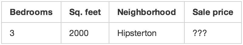
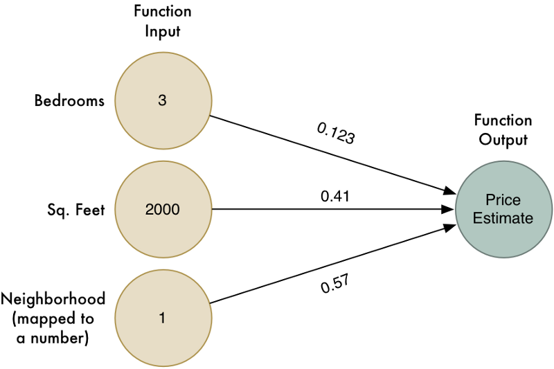
Part 1에서, 우리는 주택의 속성을 기반으로 주택 가치를 추정하는 간단한 알고리즘을 만들었습니다. 어떤 주택에 대한 데이터가 다음과 같다고 가정해 봅시다:

우리는 간단한 추정 함수(estimation function)를 만들었습니다:

def estimate_house_sales_price(num_of_bedrooms, sqft, neighborhood):
price = 0
# 이건 한 꼬집 넣고
price += num_of_bedrooms * 0.123
# 그리고 저건 한 스픈 정도 넣고
price += sqft * 0.41
# 이건 아마도 한 줌 넣고
price += neighborhood * 0.57
return price

즉, 우리는 각 속성에 가중치를 곱하여 주택 가격을 추정했습니다. 그런 다음 이 값들을 더해서 주택의 최종 가치를 얻었습니다.

코드를 사용하는 대신, 간단한 다이어그램으로 해당 함수를 표현해 보겠습니다:

화살표에 있는 숫자가 우리 함수의 가중치 입니다.

하지만, 이 알고리즘은 입력데이터와 결과 사이에 선형(linear) 관계가 있는 단순한 문제에 대해서만 동작합니다. 주택 가격이 실제로 그렇게 단순하지 않다면 어떻게 될까요? 예를 들어, 큰 주택과 작은 주택에서는 이웃이 크게 중요 할 수 있지만 중간 크기의 집에서는 중요하지 않을 수 있습니다. 우리 모델에 이런 종류의 복잡한 세부 사항을 적용할 수 있을까요?

더 영리해지기 위해서, 우리는 각각 다른 경우에 적용되는 서로 다른 가중치를 사용해서 알고리즘을 여러 번 실행해 볼 수 있습니다:

네 가지 다른 방법으로 문제를 풀어 봅시다.

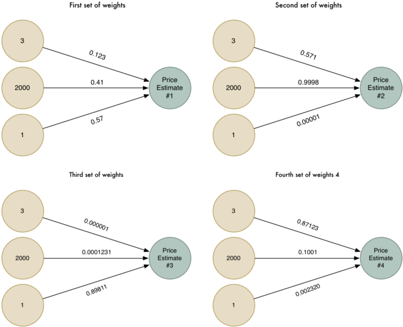
이제 서로 다른 네가지의 가격 예측이 있습니다. 이 네 가지 가격 예측들을 하나의 최종 예측으로 결합해 보겠습니다. 동일한 알고리즘으로 다시 실행할 것입니다 (다만, 다른 가중치의 세트 사용해서)!

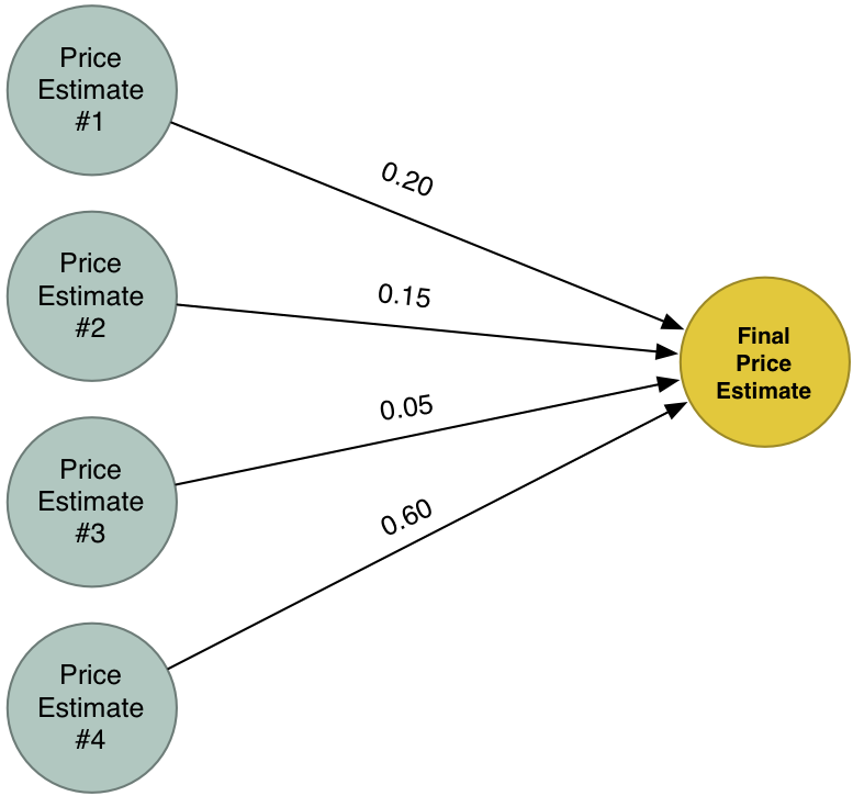
우리의 새로운 최종 해답은 문제를 해결하기위한 네 가지 시도의 예측들을 결합한 것입니다. 이러한 방법을 이용하면, 하나의 간단한 모델에서 다룰 수 있는 것보다 더 많은 사례에 대한 모델링 할 수 있습니다.

신경망(Neural Network)이란 무엇인가요?

우리의 네가지 시도를 하나의 큰 다이어그램으로 결합해 보겠습니다.

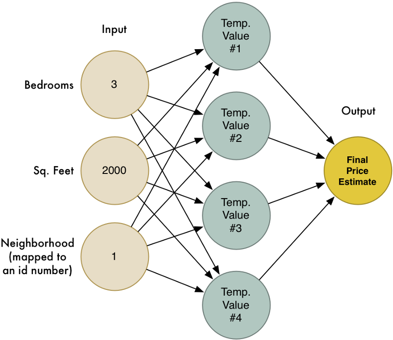
이것이 바로 신경망(neural network)입니다! 각 노드는 일련의 입력을 받아 들여 가중치를 적용하고, 출력 값을 계산하는 방법을 알고 있습니다. 이렇게 많은 노드를 서로 연결함으로써, 우리는 복잡한 함수를 모델링 할 수 있습니다.

이 글을 쉽게 유지하기 위해서 (feature scalingactivation function을 포함해서) 많은 부분을 건너 뛰었지만, 여기서 가장 중요한 것은 다음의 기본 아이디어입니다.

  • 우리는 일련의 입력을 받고 가중치를 곱해 출력을 얻는 간단한 추정 함수를 만들었습니다. 이 간단한 함수를 뉴런(neuron)이라고 부르겠습니다.
  • 단순한 뉴런들(neurons)을 서로 연결함으로써, 우리는 하나의 단일 뉴런으로 모델링하기에는 너무 복잡한 함수를 모델링 할 수 있습니다.

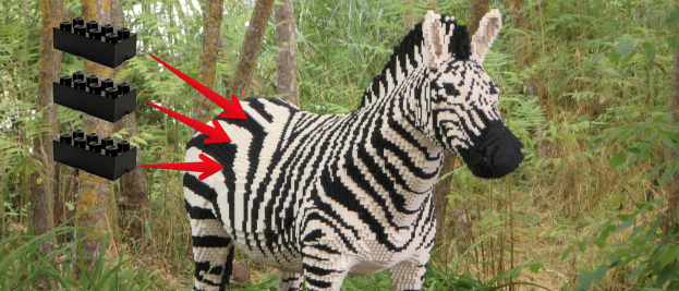
이것은 LEGO와 같습니다! 하나의 LEGO 블록으로는 많은 모델을 만들 수는 없지만, 조립할 수 있는 기본 LEGO 블록이 충분하다면 어떤 것이라도 모델링 할 수 있습니다.

이 엄숙한 플라스틱 동물의 미래는? 시간만이 알 수 있겠죠…

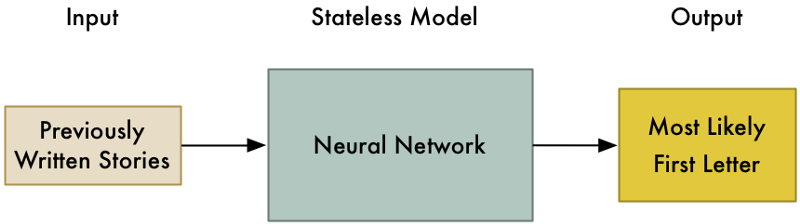
신경망(Neural Network)에 메모리 주기

앞서 우리가 본 신경망은 동일한 입력을 주면 항상 같은 결과을 반환합니다. 메모리(기억 장치)가 없기 때문입니다. 프로그래밍 용어로 말하면, 이것은 상태 비저장 알고리즘(stateless algorithm)입니다.

(집값 추정과 같은) 많은 경우에, 이 방식은 당신이 정확히 원하는 것입니다. 그러나 이런 종류의 모델이 할 수없는 한 가지는 시간이 지남에 따라 변하는 데이터의 패턴에 대응하는 것입니다.

제가 키보드를 건네주고 당신에게 이야기를 하나 써보라고 하는 상황을 상상해보십시오. 그런데 시작하기 전에, 내 직업은 사람들이 타이핑 할 첫 번째 글자를 예측하는 것입니다. 어떤 글자를 예측해야 할까요?

저는 제 영어 지식을 사용해서 올바른 글자를 예측하는 확률을 높일 수 있습니다. 예를 들어, 당신은 단어의 첫글자에 많이 사용되는 글자를 입력할 지도 모릅니다. 만약 당신이 과거에 쓴 이야기를 봤다면, 아마도 이야기의 시작 부분에서 일반적으로 사용하는 단어를 바탕으로 좀더 좁힐 수도 있을 것입니다. 일단 모든 데이터가 확보되면, 신경망을 구축해서 당신이 글을 시작할 때 특정 글자를 얼마나 사용할 가능성이 있는지를 모델링할 수 있을 것입니다.

우리는 모델은 아마 다음과 같을 것입니다:

이제 문제를 좀 더 어렵게 만들어 보겠습니다. 당신의 이야기의 어느 부분에서든 입력 할 다음 글자를 추측해야 한다고 가정해 봅시다. 훨씬 더 흥미로운 문제가 되었습니다.

어니스트 헤밍웨이(Ernest Hemingway)의 The Sun Also Rises의 처음 몇 단어를 예로 들어 보겠습니다.

Robert Cohn was once middleweight boxi

자 다음에 올 글자는 무엇일까요?

당신은 ‘n’을 추측했을 것입니다 — 그 단어는 아마도 boxing 일 것입니다. 우리는 저 문장에서 보이는 글자들과 영어의 일반적인 단어에 대한 지식을 바탕으로 이를 알 수 있습니다. 또한, ‘미들급’(‘middleweight’)이라는 단어는 권투에 대해 이야기하고 있다는 추가 단서를 제공해 줍니다.

신경망으로이 문제를 해결하려면, 우리 모델에 상태(state)를 추가해야합니다. 우리가 신경망에 응답을 요청할 때마다 우리는 중간 계산 결과들을 저장하고 다음 입력의 일부로써 다시 사용할 수 있습니다. 그렇게 하면, 우리 모델은 최근의 입력을 기반으로 예측을 조정하게 됩니다.
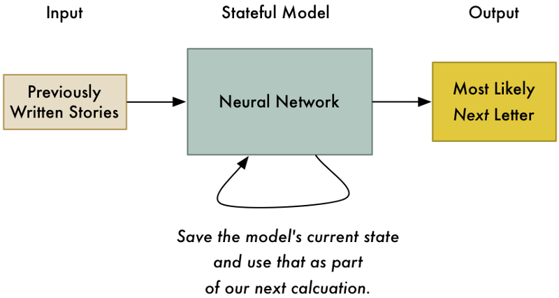
우리 모델에서 상태를 기록해 두면 단지 그 이야기에서 가장 가능성있는 글자를 예측하는 것이 아니라 이전의 모든 문자를 고려해서 가장 가능성있는 다음 글자를 예측할 수 있게 됩니다.

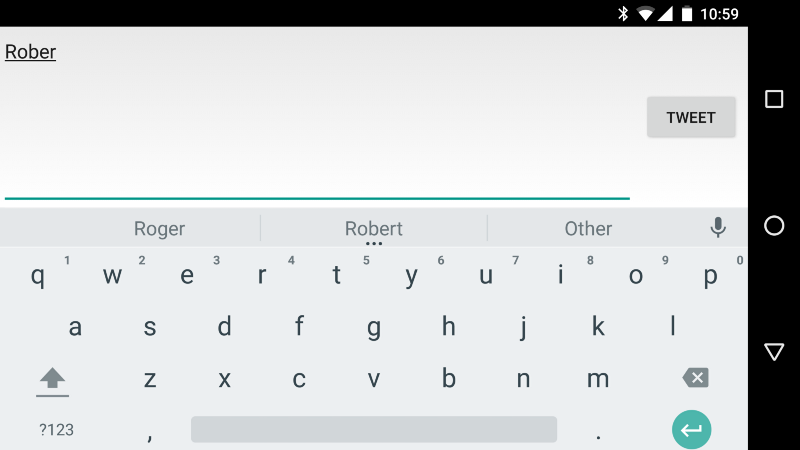
글자 하나 예측하는게 무슨 소용이 있나요?

이야기 안에서 다음 글자를 예측하는 것은 꽤 쓸모없는 것처럼 보일 수 있습니다. 여기서 중요한 것은 무엇인가요?

멋진 예 중에 하나가 바로 휴대 전화 키보드에 있는 자동 예측(auto-predict) 기능입니다:

다음 글자는 아마도 “t”가 되겠죠.

이제 이 아이디어를 극단적 끌고 가면 어떻게 될까요? 모델에 다음으로 가장 가능성있는 글자를 계속해서 아니 영원히 예측 해달라고 요청하면 어떻게 될까요? 차라리 완전한 이야기를 하나 만들어 달라고 요청하는 편이 낫겠네요!

이야기 만들기

우리는 헤밍웨이의 다음 문장을 어떻게 추측 할 수 있는지 알아보았습니다. 이제 헤밍웨이 스타일로 전체 이야기를 만들어 봅니다.

이를 위해, 우리는 Andrej Karpathy가 작성한 순한 신경망 구현(Recurrent Neural Network implementation)을 사용할 것입니다. Andrej는 Stanford의 Deep-Learning 연구원이며 RNN을 사용하여 텍스트를 생성에 대해 훌륭한 글을 썼습니다. github에서 이 모델에 관한 모든 코드를 볼 수 있습니다.

84개의 고유한 문자(구두점, 대문자/소문자 등 포함)를 사용해서 총 362,239 글자로 쓰여진 The Sun Also Rises 의 전체 텍스트로부터 모델을 제작할 것입니다. 이 데이터 세트는 현실에서 사용되는 전형적인 애플리케이션에 비하면 아주 적은 양입니다. 헤밍웨이의 스타일의 정말 좋은 모델을 제작하려면, 여러 번에 걸처 많은 샘플 텍스트를 사용하는 편이 훨씬 낫습니다. 뭐 이정도면 예를 들어 해보는데는 그런데로 충분해 보입니다.

이제 막 RNN을 훈련시키기 시작했기 때문에, 바로 글자를 예측하는 것은 그리 좋지 않습니다. 훈련을 100 회 반복 한 후 작성된 내용은 다음과 같습니다:

hjCTCnhoofeoxelif edElobe negnk e iohehasenoldndAmdaI ayio pe e h’e btentmuhgehi bcgdltt. gey heho grpiahe.
Ddelnss.eelaishaner” cot AAfhB ht ltny
ehbih a”on bhnte ectrsnae abeahngy
amo k ns aeo?cdse nh a taei.rairrhelardr er deffijha

단어들 사이에 가끔씩 공백이 있다는 정도는 알아냈지만, 이게 전부입니다.

1000 회 정도 반복 한 후에는 가능성이 있어 보입니다:

hing soor ither. And the caraos, and the crowebel for figttier and ale the room of me? Streat was not to him Bill-stook of the momansbed mig out ust on the bull, out here. I been soms
inick stalling that aid.
 “Hon’t me and acrained on .Hw’s don’t you for the roed,” In’s pair.”
 “Alough marith him.”

모델은 이제 기본 문장 구조의 패턴을 식별하기 시작했습니다. 문장의 끝 부분에 마침표를 찍고 심지어 묻고 답하는 대화도 추가했습니다. 몇 마디는 알아볼 수 있지만, 여전히 많은 부분이 말도 안됩니다.

그러나 수천 번의 훈련을 수행하니 꽤 괜찮아 보입니다:

He went over to the gate of the café. It was like a country bed.
 “Do you know it’s been me.”
 “Damned us,” Bill said.
 “I was dangerous,” I said. “You were she did it and think I would a fine cape you,” I said.
 “I can’t look strange in the cab.”
 “You know I was this is though,” Brett said.
 “It’s a fights no matter?”
 “It makes to do it.”
 “You make it?”
 “Sit down,” I said. “I wish I wasn’t do a little with the man.”
 “You found it.”
 “I don’t know.”
 “You see, I’m sorry of chatches,” Bill said. “You think it’s a friend off back and make you really drunk.”

이 시점에서, 알고리즘은 헤밍웨이의 짧고 직접적인 대화 방식의 기본 패턴을 감지해 냈습니다. 몇가지 문장은 대충 말이 됩니다.

실제 책에 있는 텍스트와 비교해 보겠습니다:

There were a few people inside at the bar, and outside, alone, sat Harvey Stone. He had a pile of saucers in front of him, and he needed a shave.
 “Sit down,” said Harvey, “I’ve been looking for you.”
 “What’s the matter?”
 “Nothing. Just looking for you.”
 “Been out to the races?”
 “No. Not since Sunday.”
 “What do you hear from the States?”
 “Nothing. Absolutely nothing.”
 “What’s the matter?”

한 번에 한 글자를 예측하는 패턴을 찾는 것만으로도, 우리의 알고리즘은 올바른 형식으로 그럴듯하게 보이는 산문을 재현해 냈습니다. 정말 놀라운 일입니다!

텍스트를 처음부터 완전하게 만들 필요는 없습니다. 그냥 알고리즘에 처음 몇 글자를 제공하고 스스로 다음 몇 글자 찾도록 내버려 두면 됩니다.

재미삼아, 상상의 책을 위한 가짜 책표지를 만들어 보겠습니다. 이를 위해서 “Er”, “He”및 “The S”을 시드(seed)로 해서 새로운 저자와 책제목을 만들어 보겠습니다.
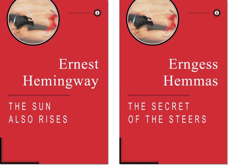
왼쪽이 진짜 책이고 오른쪽이 우리의 우스꽝스러운 컴퓨터가 만들어낸 말도 안되는 책입니다.

뭐 그런데로 괜찮네요!

그런데 정말로 놀라운 것 이 알고리즘이 모든 일련의 데이터에서 패턴을 파악할 수 있다는 점입니다. 진짜처럼 보이는 조리법이나 가짜 오바마 연설문을 쉽게 만들 수 있습니다. 그렇다면 인간의 언어에만 제한을 둘 필요가 있을까요? 아닙니다, 우리는 패턴이있는 모든 종류의 데이터에 이 아이디어를 적용 할 수 있습니다.

실제로 마리오 게임 레벨을 만들지 않고 마리오 게임 레벨 만들기

2015년, Nintendo사는 Wii U 게임 시스템 용 Super Mario Maker™를 출시했습니다.

모든 아이들의 꿈!

이 게임을 사용하면 게임패드에서 자신만의 슈퍼 마리오 브라더스(Super Mario Brothers) 레벨을 그릴 수 있고, 이를 인터넷에 업로드하면 친구들이 이 레벨을 플레이할 수도 있습니다. 자신만의 레벨에 실제 마리오 게임의 모든 기존 파워업(power-ups)과 적을 집어 넣을 수 있습니다. 이는 마치 슈퍼 마리오 브라더스를 플레이하면서 자란 사람들 위한 가상의 레고 세트와 같습니다.

가짜로 헤밍웨이의 글을 만들어낸 동일한 모델을 사용해서 가짜 슈퍼 마리오 브라더스 레벨을 만들어 낼 수 있을까요?

우선, 우리의 모델을 훈련시키 데이터 세트가 필요합니다. 1985 년에 출시 된 진짜 슈퍼 마리오 브라더스 게임의 모든 야외 레벨(outdoor levels)을 사용하겠습니다.

가장 행복한 크리스 마스. 엄마 아빠 감사해요!

이 게임에는 32개의 레벨을 있으며, 그중 대략 70%가 동일한 야외 스타일(outdoor style) 입니다. 그래서 우리는 여기에 집중하겠습니다.

각 레벨의 디자인을 얻기위해서, 게임 원본의 게임 메모리에서 레벨 디자인을 빼내는 프로그램을 작성했습니다. 슈퍼 마리오 브라더스(Super Mario Bros.)는 30년이나 된 게임이라, 레벨이 게임의 메모리에 어떻게 저장되는 지 알 수 있는 온라인 리소스가 많이 있습니다. 오래된 비디오 게임에서 레벨 데이터를 추출하는 것은 언젠가 시도해 봐야하는 재미있는 프로그래밍 연습입니다.

게임에서 추출한 첫 번째 레벨입니다 (이 게임을 해본적이 있다면 아마도 기억할 것입니다):

자세히 살펴보면 레벨은 단순한 격자 객체들로 구성되어 있음을 알 수 있습니다:

우리는 각 객체를 표현하는 문자를 사용해서 이 격자를 일련의 문자열로 쉽게 나타낼 수 있습니다.

--------------------------
--------------------------
--------------------------
#??#----------------------
--------------------------
--------------------------
--------------------------
-##------=--=----------==-
--------==--==--------===-
-------===--===------====-
------====--====----=====-
=========================-

우리는 레벨에 있는 각 객체를 문자로 대체했습니다:

  • ‘-’ 는 빈공간
  • ‘=’ 는 딱딱한 블럭
  • ‘#’ 는 깰 수 있는 벽돌
  • ‘?’ 는 코인 블럭

… 등등, 레벨에 있는 여러 객체들에 각각 다른 문자를 사용했습니다.

결과적으로 다음과 같이 텍스트 파일이 만들어 졌습니다.

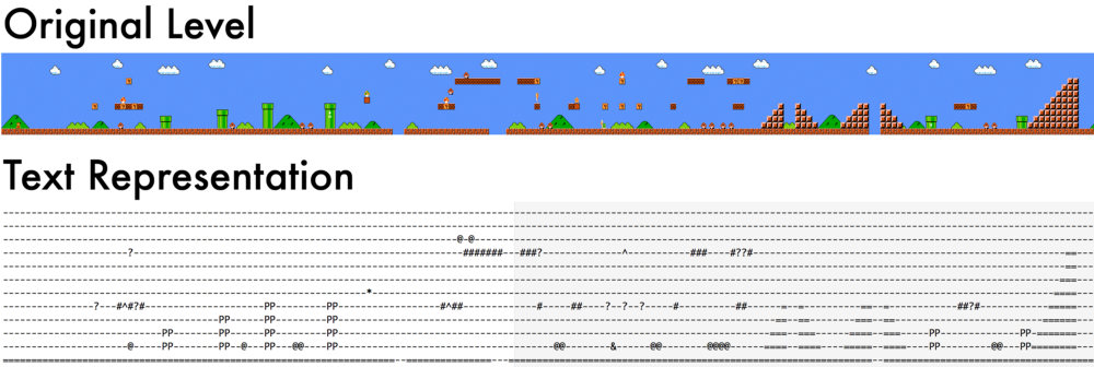
이 텍스트 파일을 살펴보면, 마리오의 레벨은 줄(line) 단위로 보면 실제로 별다른 패턴이 없다는 것을 알 수 있습니다

줄 단위로 읽어 보면 실제로 캡처할 패턴이 없습니다. 많은 줄들이 완전히 비어 있습니다.

레벨의 패턴은 레벨을 일련의 열(column)으로 생각할 때 드디어 들어나게 됩니다.

열 단위로 보면 실제 패턴이 있습니다. 예를 들어, 각 열은 ‘=’로 끝납니다.

따라서 알고리즘이 데이터에서 패턴을 찾을 수 있게 하기 위해서는 데이터를 열별로 제공(feed)해야합니다. 입력 데이터의 가장 효과적인 표현을 찾는 것(feature selection이라고 함)은 기계 학습 알고리즘을 잘 사용하기 위한 중요한 요소 중에 하나입니다.

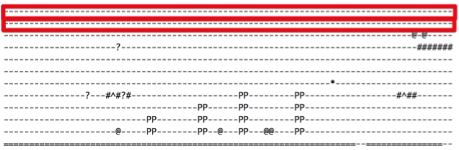
모델을 훈련시키기 위해서, 텍스트 파일을 90도 회전해야 했습니다. 이를 통해 패턴이 보다 쉽게 들어나는 순서에 따라 모델에 문자열을 제공(feed)할 수 있었습니다.

-----------=
-------#---=
-------#---=
-------?---=
-------#---=
-----------=
-----------=
----------@=
----------@=
-----------=
-----------=
-----------=
---------PP=
---------PP=
----------==
---------===
--------====
-------=====
------======
-----=======
---=========
---=========

모델 훈련시키기

헤밍웨이의 산문을 위한 모델을 만들 때 확인했듯이, 훈련시킬 수록 모델은 향상됩니다.

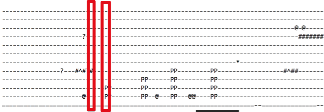
약간의 훈련 후, 우리 모델은 아직 쓸모없는 것을 만들고 있습니다:

--------------------------
LL+<&=------P-------------
--------
---------------------T--#--
-----
-=--=-=------------=-&--T--------------
--------------------
--=------$-=#-=-_
--------------=----=<----
-------b
-

현재는 ‘-’와 ‘=’가 많이 나타나야 한다와 같은 생각을 가지고 있지만, 그 뿐입니다. 아직 패턴을 전혀 알아 내지 못했습니다

수천 번의 반복을 진행하자, 이제 다음과 같은 걸 보기 시작합니다:

--
-----------=
----------=
--------PP=
--------PP=
-----------=
-----------=
-----------=
-------?---=
-----------=
-----------=

이제 모델은 각 줄이 동일한 길이여야한다는 것을 거의 알아 냈습니다. Mario의 로직 일부를 이해하기 시작했습니다: 마리오에서 파이프는 항상 2 블럭 넓이이고 높이는 최소 2 블럭 이상이므로 데이터에 “P”들은 2x2 클러스터로 나타나야 합니다. 굉장히 멋지군요!

*역자주: 여기서 2x2 클러스터란 “P”는 2글자 이상이 붙어서 두 줄에 걸처 연결된 형태(cluster)로 나타나야 한다는 의미

더 많은 훈련을 하면, 모델은 결국 완벽하게 유효한 데이터를 생성하게 됩니다:

--------PP=
--------PP=
----------=
----------=
----------=
---PPP=---=
---PPP=---=
----------=

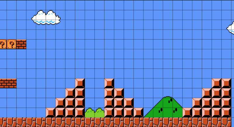
모델에서 만들어진 전체 레벨의 가치 있는 데이터를 가져와 수평으로 회전시켜 보겠습니다:

우리 모델로 만든 전체 레벨!

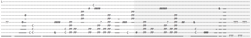
이 데이터는 정말 멋집니다! 그리고 대단한 것들이 몇 가지 있습니다.

  • 진짜 마리오 레벨처럼 Lakitu(구름을 타고 떠다니는 괴물)를 레벨의 시작되는 하늘에 집어 넣습니다.
  • 파이프는 그냥 공중에 떠 있는 것이 아니라 반드시 딱딱한 블럭들 위에 있어야 한다는 것을 알고 있습니다.
  • 적절한 장소에 적을 배치합니다.
  • 플레이어가 앞으로 나아갈 수 없도록 막는 어떠한 것도 만들지 않습니다.
  • 게임에 들어 있는 실제 레벨에서 그 스타일을 따왔기 때문에, 슈퍼 마리오 브라더스 1의 실제 레벨 같이 느껴집니다.

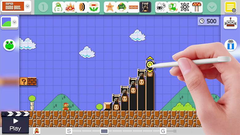
자 이제, 이 레벨을 가져와 Super Mario Maker에서 재현해 보겠습니다:
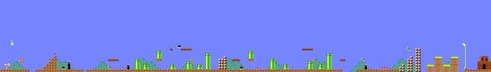
Super Mario Maker 속으로 들어온 우리의 레벨 데이터

이제 직접 플레이 해보세요!

Super Mario Maker를 사용하는 경우 온라인으로 북마크하거나 레벨 코드 4AC9–0000–0157-F3C3을 사용하여 찾아보면 이 레벨을 직접 플레이 할 수 있습니다.

장난감 vs. 실제 애플리케이션

우리가 모델을 훈련시키는데 사용한 순환 신경망(recurrent neural network 또는 RNN) 알고리즘은 실제 회사에서 음성 인식이나 번역과 같은 어려운 문제를 해결하는 데 사용하는 알고리즘과 같은 종류입니다. 우리 모델이 최첨단이 아닌 ‘장난감’으로 보이는 이유는 단지 매우 적은 데이터로 생성되었기 때문입니다. 초기 슈퍼 마리오 브라더스 게임은 정말 좋은 모델을 만들기 위한 충분한 데이터를 제공할 만큼 많은 레벨이 없을 뿐입니다.

닌텐도가 보유하고 있는 수십만 개의 사용자 제작 Super Mario Maker 레벨에 접근할 수 있다면, 우리는 정말 놀라운 모델을 만들 수도 있습니다. 그러나 닌텐도가 이를 제공하지 않기 대문에 불가능합니다. 대기업들은 데이터를 무료로 제공하지 않습니다.

더 많은 산업 분야에서 기계 학습이 더욱 중요해 짐에 따라, 좋은 프로그램과 나쁜 프로그램의 차이는 모델을 훈련시키는 데 얼마나 많은 양의 데이터를 확보했느냐가 될 것입니다. 그렇기 때문에 Google이나 Facebook과 같은 회사들이 그렇게도 여러분의 데이터를 좋아하는 것입니다.

예를 들어, Google은 대규모 기계 학습 애플리케이션을 구축하기 위한 소프트웨어 툴킷인 TensorFlow를 오픈소스로 공개했습니다. Google이 이처럼 중요하고 뛰어난 기술을 무료로 제공 한 것은 꽤나 큰 사건이었습니다. 이는 Google Translate을 강력하게 하기 위해 이를 공개했던 이유와 같습니다.

*역자주: 오픈소스를 통해 많은 사람이 사용하면 수많은 훈련 데이터가 축적되어 그 프로그램의 성능이 당연히 강력해지기 때문입니다.

즉, Google이 수집한 모든 언어에 대한 대규모 데이터가 없다면, 당신은 절대 Google Translate에 대한 경쟁 제품을 만들 수 없습니다. 데이터야 말로 Google의 가장 큰 장점입니다. 나중에 Google 지도 위치 기록(Google Maps Location History) 또는 Facebook 위치 기록(Facebook Location History)을 열어보면 당신이 이전에 가봤던 모든 장소가 저장되어 있다는걸 알게 될 것입니다.

추가 읽을 거리

기계 학습에서 문제를 해결할 수있는 유일한 방법은 없습니다. 어떻게 데이터를 사전 처리할지 또는 어떤 알고리즘을 사용할지 결정할 때 우리에겐 무한한 옵션이 있습니다. 때때로 여러 접근방법을 결합하면 하나의 접근 방법보다 더 나은 결과를 얻을 수 있습니다.

이 글을 읽은 분들이 슈퍼 마리오 레벨을 생성하는 또다른 흥미로운 접근 방법에 대한 링크들을 보내왔습니다.


Posted by uniqueone
,
https://github.com/ujjwalkarn/Machine-Learning-Tutorials/blob/master/README.md


Machine Learning & Deep Learning Tutorials Awesome

Table of Contents

Miscellaneous

Interview Resources

Artificial Intelligence

Genetic Algorithms

Statistics

Useful Blogs

Resources on Quora

Kaggle Competitions WriteUp

Cheat Sheets

Classification

Linear Regression

Logistic Regression

Model Validation using Resampling

Deep Learning

Natural Language Processing

Computer Vision

Support Vector Machine

Reinforcement Learning

Decision Trees

Random Forest / Bagging

Boosting

Ensembles

Stacking Models

Vapnik–Chervonenkis Dimension

Bayesian Machine Learning

Semi Supervised Learning

Optimization

Other Tutorials

Posted by uniqueone
,
Noninvasive Electroencephalogram Based Control of a Robotic Arm for Reach and Grasp Tasks

http://www.nature.com/articles/srep38565
Posted by uniqueone
,
https://github.com/jakevdp/PythonDataScienceHandbook


Posted by uniqueone
,
무료 온라인 파이썬(Python) 한글 교재(빠릿베짱이)

파이썬을 공부하기 위한 강좌같은 교재, 무료라서 더 Good!!!

* 파이썬(Python) 교재 : http://byteofpython-korean.sourceforge.net/byte_of_python.html

* PDF(한글) : http://byteofpython-korean.sourceforge.net/byte_of_python.pdf

* PDF(영문) : http://files.swaroopch.com/python/byte_of_python.pdf

* 출처 : http://sijoo.tistory.com/m/282

※ Table of Contents

1. 책머리

2. 헌정

3. 서문

4. 소개

5. 설치

6. 첫 걸음

7. 기초

8. 연산자와 수식

9. 흐름 제어

10. 함수

11. 모듈

12. 자료 구조

13. 실생활 문제 해결

14. 객체 지향 프로그래밍

15. 입력과 출력

16. 예외 처리

17. 표준 라이브러리

18. 더 많은 것들

19. 부록: FLOSS

20. 부록: 끝맺음

21. 부록: History Lesson

22. 부록: 변경 기록

23. 부록: 리비전 기록

24. 번역

25. 번역 방법

*********************************************************
- 통계분석연구회
- 카페 : http://cafe.daum.net/statsas
- 통계분석연구회(Statistics Analysis Study) 그룹 :https://www.facebook.com/groups/statsas

#통계 #빅데이터 #통계분석연구회 #데이터과학자 #bigdata #dataviz #statistics #Analytics
Posted by uniqueone
,
http://blogs.mathworks.com/headlines/2016/07/12/how-deep-learning-enabled-microscopy-can-detect-cancer-and-improve-biofuels/?s_eid=PSM_gen

This AI-augmented microscope uses deep learning to take on cancer 1
Posted by Lisa Harvey, July 12, 2016

According to the American Cancer Society, cancer kills more than 8 million people each year. Early detection can boost survival rates. Researchers and clinicians are feverishly exploring avenues to provide early and accurate diagnoses, as well as more targeted treatments.

Blood screenings are used to detect many types of cancers, including liver, ovarian, colon and lung cancers. Current blood screening methods typically rely on affixing biochemical labels to cells or biomolecules. The labels adhere preferentially to cancerous cells, enabling instruments to detect and identify them. But these biochemicals can also damage the cells, leaving them unsuitable for further analyses.

The ideal approach would not require labels… but without a label, how can you get an accurate signal or any signal at all?

Combining microscopy and deep learning to diagnose cancer

To address this, researchers are developing new approaches using label-free techniques, where unaltered blood samples are analyzed based on their physical characteristics. Label-free cell analysis also faces limitations: The method can damage cells, due to the intense illumination required. Label-free cell analysis can also be highly inaccurate since it often relies on a single physical attribute. New research aims to improve accuracy while minimizing damage to cells.

In a recent issue of Nature Scientific Reports, a multidisciplinary team of UCLA researchers combined a new form of microscopy called photonic time-stretch imaging with deep learning. With this powerful new technique, they were able to capture 36 million video frames per second. (Compare that rate to human vision: We can theoretically process 1000 separate frames per second, but our brains blur images into motion at speeds high than 150 frames/second. Most television and films run at 24 frames/second.) They then used these images to detect cancerous cells.


UCLA Dr. Claire Chen with microscope
Dr. Claire Chen with microscope in UCLA lab

.

The team at UCLA: A multidisciplinary approach

The team’s strategy was to devise a new and accurate label-free methodology by developing and integrating three key components into one system: quantitative phase imaging, photonic time stretch, and deep learning enabled by big imaging data analytics. All three components were developed using MATLAB.

The study was led by Bahram Jalali, UCLA professor and Northrop-Grumman Optoelectronics Chair in electrical engineering; Claire Lifan Chen, a UCLA doctoral student; and Ata Mahjoubfar, a UCLA postdoctoral fellow.

photonic time stretch diagram, UCLA
Time-stretch quantitative phase imaging and analytics system. Image credit: Claire Lifan Chen et al./Nature Scientific Reports.

Part 1: Quantitative phase imaging


The microscope uses rainbow pulses of laser light, where distinct colors of light target different locations, resulting in space-to-spectrum encoding. Each pulse lasts less than one billionth of a second. The ultrashort laser pulses freeze the motion of cells, giving blur-free images. The photons with different wavelengths (colors) carry different pieces of information about the cells.

As the photons travel through the cells, the information about the spatial distributions of the cells’ protein concentrations and biomasses are encoded in the phase and amplitude of the laser pulses at various wavelengths. This information is later decoded in the big data analytics pipeline and used by the artificial intelligence algorithm to accurately identify cancerous cells without any need for biomarkers.

The microscope also uses low illumination and post-amplification. This solves the common problem in label-free cell analysis, where the illumination used to capture the images destroys the cells.

“In our system, the average power was a few milliwatts in the field of view, which is very safe for the cells,” stated Claire Lifan Chen. “But, after passing through the cells, we amplify the signal by about 30 times in the photonic time stretch.”

Specially designed optics improve image clarity in this microscope. The researchers have used MATLAB to design the microscope according to the resolution requirements in their biomedical experiments. Image reconstruction and phase recovery are also designed in MATLAB for further downstream analysis.

Part 2: Amplified time-stretch system


Photonic time stretch, invented by Professor Jalali, transforms the optical signals and slows the images so that the microscope can capture them. The microscope can image 100,000 cells per second. The images are digitized at a rate of 36 million images per second, equivalent to 50 billion pixels per second.

The photons travel through a long, specialized fiber and arrive at the sensors during the time between laser pulses. MATLAB was used to determine the parameters for this dispersion compensating fiber.

“The system adds different delays to the pixels within a pulse and feeds them one-by-one, serially, into the photodetector,” said Ata Mahjoubfar.

A software implementation of the physics behind phase stretch transform (PST) as an image feature detection tool from the UCLA Jalali Lab is available for download from MathWorks File Exchange. The code uses Image Processing Toolbox.

The PST code is also available on Github: It has downloaded or viewed more about 27,000 times since May. At the time of this post, it has the third highest star rating of the current MATLAB repositories.


UCLA Microscope in Lab
Artificial-intelligence time-stretch microscope.

Part 3: Big data analytics using deep learning


Once the microscope captures the images, the team used domain expertise to extract 16 biophysical features of the cells, such as size and density. Recording these features is like documenting the fingerprints of each individual cell. This method yields a high-dimensional dataset which is used to train the machine learning application for identifying cancer cells.

With millions of images to analyze, the team turned to machine learning to solve the multivariate problems. Using MATLAB, the authors implemented and compared the accuracy of multiple machine learning approaches ranging from Naive Bayes and Support Vector Machines, to Deep Neural Network (DNN).

The approach that provided the best performance was a custom DNN implementation that maximized the area under ROC curve (AUC) during training. The AUC is calculated based upon the entire data set, providing inherently high accuracy and repeatability. The success of DNNs for this challenging problem is derived from their ability to learn complex nonlinear relationships between input and output.

In comparing the performance of various classification algorithms, the DNN AUC classifier provided an accuracy of 95.5 % compared to 88.7 % for a simple Naive Bayes classifier. For applications like cancer cell classification, where implications of positive or negative diagnosis are so high, this improvement in accuracy highly impacts the usability of a method.

The more images provided, the more accurate the training system can become. The team trained the machine learning model with millions of line images and used parallel processing to speed up the data analytics. Using high-performance computing (HPC), the image processing and deep learning can be readily performed in real-time by an online learning configuration.

The language of innovation


Not content with simply developing a new microscopy technique, the team utilized the augmented microscope to detect cancer cells more accurately and in less time than current techniques. They also were able to determine which strains of algae provide the most lipids for subsequent refining into biofuels. Yes, one methodology that tackled both biofuels and cancer.

Innovation cannot be achieved without creativity, inspiration, and dedication. Having an interdisciplinary team also helps: This work was a result of collaborations between computer scientists, electrical engineers, bioengineers, chemists, and physicians.

“As we were developing our artificial-intelligence microscope, we crossed the boundaries of scientific fields and modeled biological, optical, electrical, and data analytic systems interconnectedly. MATLAB is a great language for prototyping and provided cohesion to this process, ” said Ata Mahjoubfar.
And, as these researchers demonstrate so eloquently in their publication, having a single language of innovation can facilitate collaboration and accelerate innovation amongst various disciplines in science and engineering.

You can find this and other useful community-developed tools for microscopy here.
Posted by uniqueone
,
https://docs.google.com/spreadsheets/d/1AQvZ7-Kg0lSZtG1wlgbIsrm90HaTZrJGQMz-uKRRlFw/htmlview#
Posted by uniqueone
,
google find  "svm parameter optimization matlab"


http://www.mathworks.com/help/releases/R2013a/stats/support-vector-machines-svm.html#bsr5o1q


https://www.mathworks.com/matlabcentral/answers/63535-using-fminsearch-to-optimize-svm-parameters


https://www.mathworks.com/matlabcentral/answers/124635-finding-best-parameters-of-svm


https://www.mathworks.com/matlabcentral/answers/78466-how-to-customize-svm-kernel-parameters-in-matlab?s_tid=answers_rc1-2_p2_MLT


https://www.researchgate.net/post/How_can_I_tune_a_SVM_classifier_in_Matlab


google image find "cross validation parameter tuning"


http://online.cambridgecoding.com/notebooks/cca_admin/scanning-hyperspace-how-to-tune-machine-learning-models


http://online.cambridgecoding.com/notebooks/cca_admin/misleading-modelling-overfitting-crossvalidation-and-the-biasvariance-tradeoff


https://www.facebook.com/search/top/?init=quick&q=%EC%B0%B8%EA%B3%A0%EB%A1%9C%20ML%20%EB%B6%84%EC%95%BC%EB%8A%94%20%EA%B1%B0%EC%9D%98%20%EC%B4%88%EC%8B%AC%EC%9E%90%20%EC%88%98%EC%A4%80%EC%9E%85%EB%8B%88%EB%8B%A4&tas=0.9154726614105413


Posted by uniqueone
,
https://www.opendatascience.com/blog/learning-reinforcement-learning-with-code-exercises-and-solutions/?utm_source=Open+Data+Science+Newsletter&utm_campaign=63677c26f2-EMAIL_CAMPAIGN_2016_12_13&utm_medium=email&utm_term=0_2ea92bb125-63677c26f2-245860601


Open Data Science
Toggle navigation
Learning Reinforcement Learning (With Code, Exercises and Solutions)


By Denny Britz, Deep Learning Specialist - Google Brain | 12/14/2016
Tags: Algorithms

Skip all the talk and go directly to the Github Repo with code and exercises.

WHY STUDY REINFORCEMENT LEARNING

Reinforcement Learning is one of the fields I’m most excited about. Over the past few years amazing results like learning to play Atari Games from raw pixels and Mastering the Game of Go have gotten a lot of attention, but RL is also widely used in Robotics, Image Processing and Natural Language Processing.

Combining Reinforcement Learning and Deep Learning techniques works extremely well. Both fields heavily influence each other. On the Reinforcement Learning side Deep Neural Networks are used as function approximators to learn good representations, e.g. to process Atari game images or to understand the board state of Go. In the other direction, RL techniques are making their way into supervised problems usually tackled by Deep Learning. For example, RL techniques are used to implement attention mechanisms in image processing, or to optimize long-term rewards in conversational interfaces and neural translation systems. Finally, as Reinforcement Learning is concerned with making optimal decisions it has some extremely interesting parallels to human Psychology and Neuroscience (and many other fields).

With lots of open problems and opportunities for fundamental research I think we’ll be seeing multiple Reinforcement Learning breakthroughs in the coming years. And what could be more fun than teaching machines to play Starcraft and Doom?

HOW TO STUDY REINFORCEMENT LEARNING

There are many excellent Reinforcement Learning resources out there. Two I recommend the most are:

David Silver’s Reinforcement Learning Course
Richard Sutton’s & Andrew Barto’s Reinforcement Learning: An Introduction (2nd Edition) book.
The latter is still work in progress but it’s ~80% complete. The course is based on the book so the two work quite well together. In fact, these two cover almost everything you need to know to understand most of the recent research papers. The prerequisites are basic Math and some knowledge of Machine Learning.

That covers the theory. But what about practical resources? What about actually implementing the algorithms that are covered in the book/course? That’s where this post and the Github repository comes in. I’ve tried to implement most of the standard Reinforcement Algorithms using Python, OpenAI Gym and Tensorflow. I separated them into chapters (with brief summaries) and exercises and solutions so that you can use them to supplement the theoretical material above. All of this is in the Github repository.

Some of the more time-intensive algorithms are still work in progress, so feel free to contribute. I’ll update this post as I implement them.

TABLE OF CONTENTS

Introduction to RL problems, OpenAI gym
MDPs and Bellman Equations
Dynamic Programming: Model-Based RL, Policy Iteration and Value Iteration
Monte Carlo Model-Free Prediction & Control
Temporal Difference Model-Free Prediction & Control
Function Approximation
Deep Q Learning (WIP)
Policy Gradient Methods (WIP)
Learning and Planning (WIP)
Exploration and Exploitation (WIP)
LIST OF IMPLEMENTED ALGORITHMS

Dynamic Programming Policy Evaluation
Dynamic Programming Policy Iteration
Dynamic Programming Value Iteration
Monte Carlo Prediction
Monte Carlo Control with Epsilon-Greedy Policies
Monte Carlo Off-Policy Control with Importance Sampling
SARSA (On Policy TD Learning)
Q-Learning (Off Policy TD Learning)
Q-Learning with Linear Function Approximation
Deep Q-Learning for Atari Games
Double Deep-Q Learning for Atari Games
Deep Q-Learning with Prioritized Experience Replay (WIP)
Policy Gradient: REINFORCE with Baseline
Policy Gradient: Actor Critic with Baseline
Policy Gradient: Actor Critic with Baseline for Continuous Action Spaces
Deterministic Policy Gradients for Continuous Action Spaces (WIP)
Deep Deterministic Policy Gradients (DDPG) (WIP)
Asynchronous Advantage Actor Critic (A3C) (WIP)
Originally posted at www.wildml.com/

WHAT IS OPEN DATA SCIENCE?

Username *

Email *

Password *

Repeat Password *
Get Newsletter & Full Access
 
LATEST POSTS
Scikit-learn Tutorial: Statistical-Learning for Scientific Data Processing
12/14/2016

Learning Reinforcement Learning (With Code, Exercises and Solutions)
12/14/2016

Visualizing the Relationship Between Infant Mortality Rates & Resource Availability
12/14/2016

 
POPULAR POSTS
Riding on Large Data with Scikit-learn
   9997 views

R or Python for data science?
   9841 views

huh Understanding Convolutional Neural Networks for NLP
   9252 views

RELATED POSTS
Introducing Dask distributed #1
09/13/2016

An Introduction to Contextual Bandits
09/06/2016

Jester Dataset: What make’s You laugh?
08/09/2016

Topnotch Theano Tutorial
02/05/2016

Single-Layer Neural Networks and Gradient Descent
09/10/2016

Ad Hoc Distributed Random Forests
09/17/2016

R-BLOGS
New Course: Data Visualization in R
Posted 14 December 2016 | 6:59 pm
R Jobs for R users – 17 jobs from around the world (2016-12-14)
Posted 14 December 2016 | 6:57 pm
One Page R: A Survival Guide to Data Science with R
Posted 14 December 2016 | 5:44 pm
Visualizing taxi trips between NYC neighborhoods with Spark and Microsoft R Server
Posted 14 December 2016 | 5:40 pm
Hierarchical Clustering exercises (beginner)
Posted 14 December 2016 | 5:00 pm
TAGS
Artificial Intelligence
Cyber Security
Analytics
Sports Analytics
Notebooks
Open Source
ipython
Anomaly Detection
Data Journalism
Computer Vision
Data Science Careers
Julia
ODSC London 2016
Data Science Jobs
Pandas
Open Data Science
Tutorial
Interview
Natural Language Processing
Politics
statistics
Meetup
NLP
Data Science for Good
Jupyter
Spark
Bayes
Data Mining
AI
Algorithms
Data analysis
IoT
Predictive Analytics
Intro
BDF 2015
Deep Learning
Scikit-learn
Open Data
Data Visualization
Neural Networks
Big Data
Speaker Talk
R
ODSC East 2016
ODSC West 2015
Speaker Slides
Python
Data Science
Machine Learning
ODSC East 2015
Copyright © 2016 Open Data Science. All rights reserved.
Privacy-policy
Code of conduct
FOLLOW US:
Posted by uniqueone
,

Random forest는 고차원 데이터에서 중요 변수를 찾기위한 방법으로 널리 이용되지만 훈련데이터의 변화에 따라 선택되는 변수군이 크게 달라지는 단점이 있다. """"또한 decision tree의 계층적 구조로 인해 ★불필요한 변수들도 함께 선택될 수 있으며★ 이런 문제는 random forest를 구성하는 tree의 수가 많아질수록 악화된다. """"""""


http://dmqm.korea.ac.kr/board/view.asp?B_CATEGORY=0&B_CODE=b_papers&tID=105&sID=122&IDX=69&gotopage=3&search_category&searchstring


발표자 Summary


박찬희

Regularized random forest (RRF)는 대표적인 앙상블 기법인 random forest에 regularized 기법을 적용한 방법이다. Random forest는 고차원 데이터에서 중요 변수를 찾기위한 방법으로 널리 이용되지만 훈련데이터의 변화에 따라 선택되는 변수군이 크게 달라지는 단점이 있다. 또한 decision tree의 계층적 구조로 인해 불필요한 변수들도 함께 선택될 수 있으며 이런 문제는 random forest를 구성하는 tree의 수가 많아질수록 악화된다. RRF에서는 각 노드에서 관측치를 분할시킬 변수 선택시 기존에 선택되었던 변수들외에 새로운 변수의 information gain값에 패널티를 부가 하게 된다. 이를통해 random forest보다 적은 변수군으로 모델을 구성할 수 있다. 하지만 tree모델은 greedy search를 기반으로 하기 때문에 RRF는 변수 중요도 보다 먼저 선택된 변수들 위주로만 중요 변수군이 만들어진다는 단점이 있다.이를 보완하기 위해 guided regularized random forest (GRRF)가 제안되었다. GRRF는 새로운 변수의 gain값에 패널티를 부과시 변수의 중요도가 높을 수록 낮은 패널티 값을 부과한다.

따라서 기존에 선택되지 않은 변수라도 중요도가 높으면 중요 변수군에 포함될 수 있게 된다. RRF와 GRRF 분류모델은 최소한의 변수군으로 모델이 구성되기 때문에 random forest에 비해 높은 variance를 가질 수 있다. 따라서 GRRF와 RRF로 중요변수를 선택하고  random forest로 분류 모델을 구축하는 방법이 추천된다. 


청취차 Summary


유재홍

금일 세미나는 Random forest기반의 변수선택 기법을 개선한 Regularized Random Forest와 Guided Regularized Random Forest를 주제로 진행되었다. 이 두 기법은 Random forest에서 중요하다고 판단되는 변수가 지속적으로 선택되도록 Information Gain에 대해 가중치를 주도록 하는 방법이다. 이 기법을 적용하면 일관적으로 변수가 선택된다는 장점이 있지만, 중요변수가 계속해서 선택되므로 개별 모델 간 상관성이 높아져서 모델의 Variance가 증가한다는 한계점도 존재한다. 또한, 중요하다고 판단되는 변수만을 지속적으로 선택하게 함으로써 지역최적화에 빠지게 될 수도 있다는 위험도가 높지 않을까 생각된다. 특히, Guided Regularized Random Forest의 경우에는 일반적인 Random Forest를 구축하고 이를 바탕으로 변수의 중요도를 계산하여 이를 바탕으로 Regularized Random Forest의 가중치를 구하게 되는데, 이러한 경우, 최종적으로 구축된 모델이 초기의 Random Forest 모델에 대해 Bias될 수도 있겠다는 생각이든다. 나 역시 앙상블 기법를 기반으로 하여 군집화를 위한 변수선택을 연구하고 있는데, 이 기법에 대해 좀 더 심도있게 공부해야 겠다는 생각이 들었다.


남완식

오늘 세미나는 오리지널 Random Forest 알고리즘에 Regularized 개념을 접목하여 모델의 안정성을 더욱 높여준 RRF(Regularized RF)와 RRF 알고리즘의 Variable Selection 신뢰성을 더욱 높여준 GRRF(Guided RRF) 알고리즘에 대한 설명으로 진행되었다. 본인이 개인적으로 학습하며 느꼈던 가려운 부분을 제대로 긁어준 좋은 시간이었다. 세미나에서 박찬희 연구원이 언급했던 것처럼 새로운 Penalty Term으로 기존 RRF나 GRRF 보다 우수한 성능을 보여줄 알고리즘에 대한 기대가 크다. 꼭 기존 보다 더 우수한 성능을 보이지 않더라도 새로운 Penalty Term이 기존 연구와 동일한 성능만 보여줘도 충분히 좋은 결과라고 생각된다. 앞으로의 연구에 기대와 응원을 하며 후기를 마친다.


최우식

개인적으로 랜덤 포레스트의 몇몇 단점 때문에 좀 더 개선된 방식의 알고리즘이 없을까 궁금하였는데, 이번 세미나를 통해 쉽고 빠르게 궁금증을 해소할 수 있었다. 사실 랜덤 포레스트는 현재 연구실에서 자주 사용하고 있는 데이터마이닝 알고리즘 중에서도 최신 기법이라 할 수 있는데, 그럼에도 불구하고 다양한 개선 방법이 나오고 있다는 점 자체가 본인에게는 충분히 자극제가 되겠다. 세미나에서 제시된 GRRF (guided regularized random forest)는 데이터에서 유의미한 변수를 잘 추출하는 것이 핵심이므로, 이를 개인적으로도 다양한 방식으로 활용할 수 있을 것이다. 추가로, GRRF에는 사용자가 지정할 수 있는 파라미터가 두 개 존재하는데, 이를 보다 효과적으로 지정하는 것도 좋은 연구가 될 수 있겠다고 생각하였다.


박영준

금일 세미나는 찬희형이 guided regularized random forest (GRRF)에 대해 설명하였다. 이 모델은 기존의 random forest를 이용한 변수선택 보다 더 적은 수의 변수를 선택하여 tree를 구성하는 regularized tree를 이용하였고, 사전에 구축한 random forest의 변수 중요도를 이용하기 때문에 guided라는 표현이 붙어있다. 세미나를 통해 GRRF는 random forest에 비해 모델의 variance가 크기 때문에 classifier로서는 부적합 하고, 변수선택 모델로 사용하는 것이 낫다는 설명을 들었다. 더 적은 변수를 가지고 모델을 구성하는 경우 linear regression 에서는 variance는 줄어든다고 알고 있었는데 tree에서는 반대가 되는것이 처음에는 의아하였지만 세미나를 통해 bias-variance trade off  관계에 대해 잘 못 이해하고 있는 부분을 바로 잡을 수 있었다. 개인적으로 유익한 시간이었다. 이 기회에  모델링에서 항상 언급되는 bias-variance trade off를 더 공부해 봐야 겠다.


정영재

찬희 형의 "Introduction to Guided Regularized Random Forest"라는 주제의 세미나를 들었다. Essemble Model의 일종인 Random Forest는 변수선택에 있어서 변동(variance)가 크다. 이 문제를 Lasso에서는 Penalty Term을 설정함으로서 해결하였기 때문에, Guided Random Forest(GRF)에서는 이를 응용하여 Impurity Measure에 Penalty Term을 준 방법으로, 변수선택에 목적이 있다. 즉, GRF에서 변수를 선택한 후, 그 변수만으로 Random Forest 기법을 써서 분류를 하면 변수선택의 변동이 줄어듬과 동시에 성능(Error Rate)가 줄어듬을 확인할 수 있었다. 동시에 다른 Feature Selection 기반 Random Forest보다 계산시간도 적었다. Random Forest에 Lasso의 Penalty Term을 응용한 방법이 흥미로웠다. GRF에 의해 선택된 변수들이 Random Forest말고 다른 분류기법에도 잘 적용되는지, 또는 다른 변수선택 기법 기반으로 Random Forest기법 사용시 성능이 어떠한지 알아보는 것도 좋을 것 같다.


손지은

기존의 Regularized Random Forest 의 한계점을 보완하기 위해 연구 된 Guided Regularized Random Forest(GRRF)를 소개하였다.패널티를 계산할 때, importance score를 추가해줌으로써 변수의 중요도를 고려하여 random 선택할 수 있도록 한것이 연구의 핵심이었다.그러나 importance score 의 가중치를 결정하는 gamma가 user parameter 인데, 실험 결과에서 오히려 gamma값의 영향이 미미한것 같아 좀 의문이었다.


이한규

오늘의 세미나는 Guided Regularized Random Forest(GRRF)에 관한 내용으로 Random Forest를 이용한 classification문제라기 보단 classification에 앞서서 Featrue selection에 관련된 내용이었다. 일반적으로 Random Forest의 경우 변수선택과 동시에 classification이 가능하다고 알려져 있으나 변수를 선택함에 있어서 선택된 변수들의 variance가 높은 경향을 보인다. 이를 개선하기 위한 방법으로써 regularized method를 활용하여 변수를 기존의 방식보다 compact하게 선택하는 방법이었다. 

점차 고차원의 데이터를 분석함에 따라, Regularized method를 익히는 것 그리고 그에 파생된 다양한 기법들을 익히는 것이 중요하다고 생각되는데 어떻게 보면 이번 시간를 통해 그러한 방법중 한가지라도 제대로 알게 되어 유익한 시간이었다고 생각한다. 참고로 R에서는 이미 "RRF"라는 패키지 않에 GRRF를 사용할 수 있도록 나와있어서 간단하게 example을 따라 해봄으로써 이해를 더욱 빨리 할 수 있을 것 같다. 


이슬기

지난번에 GRRF에 대해 가볍게 언급했던 세미나가 있었는데 이번 세미나에서 정확히 어떤 목적을 가지고 어떤 아이디어를 제안하여 구현한 것인지 알 수 있었다. 랜덤포레스트가 정확도가 높으면서 변수선택도 가능한 알고리즘이지만, 실제로 사용을 했었을 때 너무 많은 변수가 선택되어 중요변수를 확인하기가 어려운 적이 있었다. 실제 변수선택으로 사용하기 위해 조금 부족함이 있다고 생각이 들었는데, 조금 더 중요한 변수를 뽑는 것을 목적으로 하는 알고리즘이 이미 개발되었으므로 실제 문제를 풀 때 사용할 수 있을 것 같다. 특정한 아이디어를 제안하지는 않았지만, 기존에 있던 연구들에 대해 충분히 공부가 되어 있다는 느낌을 받았다. 자세한 내용에 하나의 알고리즘을 꾸준히 연구하는 것이 본받아야 할 자세라 생각이 든다.


강현구

오늘 세미나에서는 Guided Regularized Random Forest(GRRF)에 대한 설명을 들었다. Random Forest에서는 각 의사결정나무의 노드에서 분할 시, random subspace method를 이용하여 분할에 이용할 변수를 선택한다. 이 과정에서 불필요하게 많은 변수들이 선택되는 것을 방지하기 위하여, 한 번 사용한 변수를 이후에도 많이 사용할 수 있도록 하는 것이 GRRF이다. 성능 면에서는 일반적은 random forest보다 떨어지지만, 적은 수의 변수를 사용하기 때문에 변수 선택 기법으로 활용하는 것이 좋을 것 같다. GRRF를 통하여 선택된 변수들을 이용하여 다시 random forest 알고리즘을 실행할 수도 있다. Lasso처럼 변수 선택에 있어서 제약을 주는 기법들이 많이 등장하면서 기존의 알고리즘들과 많이 결합되는데, 페널티를 어떻게 주느냐에 따라 변수 선택의 결과도 달라질 수 있을 것 같다. 


곽민구

Decision Tree부터 오늘 세미나 주제인 GRRF까지 개념적인 설명을 잘 들을 수 있었던 세미나였습니다. 각 모델이 가지고 있는 장점과 단점을 설명해주고, 그 점들을 보완하기 위해서 나온 모델들을 순차적으로 소개해 이해에 많은 도움이 되었으나, LASSO 등 생소한 개념들이 많아 완벽하게 이해하기 어려웠습니다. 또한 Tree를 Classification 모델이 아닌 Feature Selection 모델로 사용했다는 점에서 흥미로웠습니다


박진수

얼마전 Regularized method에 이어 Guided Regularized Random Forest에 대하여 알아보는 시간을 가졌다. 앙상블모델은 정확도를 높이기 위하여 많이 쓰이는데 일반적으로 Base 모델의 오류율이 0.5보다 작을때 앙상블 모델의 오류율은 항상 그보다 작다. 특히 그 중에서도 앙상블 모델 중 하나인 Random Forest는 많이 쓰이는데, 이 Random Forest의 단점은 stability가 낮다는 것이다. 이를 보완하기 위하여 GRRF와 RRF가 제안되었는데, 개념은 새로운 변수가 선택될 가능성을 줄이는 것이다. 특출나게 좋은 변수가 아닌 이상 새로 변수를 추가하지 않고 기존의 변수를 사용하게 된다. 이를 통하여 오류율도 기존 RF보다도 적게 나왔다. 다만, 논문의 저자도 변수가 적게 선택되는 만큼 tree간에 correlation이 클 가능성이 있기 때문에 Classifier로서보다는 변수선택기법으로만 사용하라고 제안하고 있다. 즉, GRRF나 RRF로 변수를 선택하고 RF로 결과를 내는 것을 제안하고 있다. 본 발표에서는 람다와 Importance score를 사용하였는데 박찬희 연구원은 새로운 기법으로 Regularization을 해보고자 준비하고 있는 것 같다. 좋은 연구 결과가 있을 거라 기대한다.


도형록

이번 세미나는 guided regularized random forest에 대한 내용으로 진행되었다. Regularized random forest는 regularized tree에 기반한 알고리즘으로 이전 남완식 연구원의 세미나에서도 잠깐 언급되었다. Regularized decision tree는 tree에서 redundant한 변수를 사용하지 않도록 regularize 하는 방법으로, decsion tree에서 split 할 때 새로운 변수를 추가적으로 사용하지 않는 방향으로 작동한다. RRF는 각 regularized tree에서 새로운 feature와 기존 feature에 대한 가중치를 모두 동일하게 설정하는 방법이며, Guided RRF는 각 변수의 variable importance에 따라 가중치를 다르게 설정하는 방법이다. RRF나 GRRF는 변수선택에 있어서는 좋은 결과를 보이지만, 예측에 있어서는 높은 variance를 보이므로, feature selection에만 이용하는 것이 좋다고 한다. 현재 regularization 모델에 관련된 연구를 진행하고 있는데, regularization과 ensemble method를 접목하는 연구에 대해 좋은 정보를 얻게 되었다.


이상민

박찬희 연구원의 금일 발표는 Regularized method 중 Regularized ensemble methods 주요 기법들에 대한 소개가 있었다. 일반적인 regularization 하기 위한 방법으로 Lasso 기법에 대해서만 알고 있었으므로, ensemble 기반의 feature selection 기법에 대한 이해를 할 수 있어 좋은 시간이었다.금일의 세미나의 핵심은 GRRF와 RRF의 차이점을 잘 설명했던 것으로, 기존에 기존 Lasso에서 선택의 정확도를 높이기 위해 잘 선택되지 않은 변수에 대한 penalty를 주는 것과 다르게, 도입한 변수의 중요도(Important)값을 고려하여 penalty(람다값)을 data-driven 방식으로 조정하는 방식에 의한 것이다. 즉, 람다값이 사용자에 의해 고정된 값으로 주지 말고 앙상블에 의해 선택된 빈도수가 높은 변수일수록 penalty를 덜 받도록 조정해주는 방식인 것이다. 방식의 좋고 나쁨을 떠나서, 내 생각에 penalty term은 본래 의미대로 penalty 역할만을 수행하는게 좋다고 생각하므로, GRRF 외 다른 방식으로 regularization을 보정하는 방식이 있을 것이라 생각한다. 다시 말해, penalty 보정을 위해 사용해야 하는 Important score는 strong law of large numbers 에 따라 다수 선택되는 변수일 수록 중요도를 더하는 의미라면 별도의 수식으로 도출하는게 필요하다고 생각한다. 'Penalty' 와 'Important'의 의미를 0과 1 사이의 값으로 적당히 normalize한 것 외 다른 방법이 있을 것 같다. 박찬희 연구원도 분명 이러한 점을 지적하여 연구주제로 잡아서 소개해준 것 같다. 새로운 분야에 대해 입문할 수 있게 도와준 박 연구원에게 감사하다.


유화윤

Guided Regularized Random Forest에 대한 세미나였는데 여러가지 기본 개념부터 advanced 내용까지 다루어서 이해하기 어려운 점이 있었다. Ensemble의 의미가 무엇인지 몰랐었는데 이번세미나를 통해 간단히 알 수 있었고, Information Gain, Decision Tree의 변수 선택방법에 대해서는 비정형 데이터 분석 수업에서 배웠음에도 잊었는데 다시 인지하게 되어 좋았다. RF, RRF, GRRF의 차이점에 대해 배울수 있었는데 요약하면 아래와 같다. 모두 변수선택 기능이 있는데 RF는 Random으로 변수를 선택하고 Tree를 많이 하면 변수 선택이 Biased되지는 않지만 Variance가 크고 주요하지 않은변수도 뽑히는 단점이 있다. RRF는 변수의 Coefficient에 패널티를 주는데 패널티 값에 따라 이전 Tree에서 선택되지 않은 변수는 선택된 변수보다 훨씬 큰 Gain값을 갖지 않는한 선택되기 어려워서 변수가 Biased될 수 있다는 것이 단점이다. 이것을 보완하기 위해 GRRF가 사용 될 수 있는데 이것은 importance value를 추가하여 이전 tree에는 등장하지 않았지만 전체적으로 많이 사용된 변수는 선택이 더 잘 될 수 있게 한 것이다. 연구원이 계획한대로 변수을 선택할 때 한쪽으로 치우치지 않고 개수는 최소화하여 효과적으로 잘 뽑일 수 있게 하기 위해서 importance value외에도 다른 방법을 고안하는 것이 좋은 연구가 될 수 있겠다.  마지막으로 RF 계열 방법이 변수수가 관측치 수보다 많을 때 좋은 효과가 있다고 한다.  내가 갖고있는 데이터는 변수수가 적어서 그런지 Linear Regression보다 RF 결과가 좋지 않았다. 그렇지만 RRF나 GRRF로 변수를 선택하고 RF에 적용하여 변수가 적을땐 어떤 효과가 있는지 비교해보는 것도 좋겠다.


박성호

랜덤 포레스트는 대표적인 앙상블 기법으로써 Bootstrap Sampling을 통하여 데이터를 구성하며, 랜덤하게 선택한 변수들을 가지고 나무 모델의 각 노드를 구성하여 최종 나무 모델을 구축한다. 앙상블의 특성상 예측정확도 측면에서 Variance가 낮아 기계학습 알고리즘 중에서 널리 사용되고 있다. 또한, 랜덤 포레스트는 변수 선택기법으로 널리 사용되기도 한다. 하지만 랜덤하게 변수를 선택하는 특성 때문에 변수선택에 분산이 크고 많은 상대적으로 많은 변수가 뽑힌다. 이러한 점에 착안하여 변수의 사용빈도와 예측 정화도측면에서 가중치를 적용하여 변수 선택을 하여 기존 보다 좋은 성능을 보여주는 Guided Regularized 랜덤 포레스트가 연구되었다. 새로운 연구를 시작하는데 있어랜덤 포레스트에서 Guided Regularized 랜덤 포레스트까지 이어지는 연구의 흐름을 착안하여 방향성 및 시나리오 구축해보면 좋지 않을까 생각된다. 


소현진

오늘 세미나는 Guided regularized random forest에 대해 알 수 있는 유익한 시간이었다. 발표를 진행한 박찬희 연구원은 먼저 Ensemble method의 개념과 발전과정에 대해 설명하고 기존 방법에 Regulized method가 어떻게 접목되어 발전되었는지 부연하였다. 박찬희 연구원의 세미나 진행은 연구를 시작하거나 평소 관련 주제에 관심을 가지고 있는 청취자를 상당히 배려하여 진행되었다. 예를 들어, 새로운 개념이 나오면 먼저 설명한 뒤 청중에게 개념에 대해 역으로 질문을 하여 이해했는지를 확인했다. 또한 연구를 진행하다 맞닥뜨려지는 문제에 대해 질문하고 이해시킴으로써 앞선 선진 연구자의 모습을 보여주었다. 본인에게 Ensemble method는 다음 학기에 집중 연구할 분야이기 때문에 오늘 세미나는 앞으로의 연구를 위한 귀한 지침이 될 것 같다. 발표자에게 감사를 표하며 세미나 후기를 마친다.


구자연

최근 우리 연구실에서 유재홍 연구원이 앙상블 기법에 대해서 소개하고, 남완식 연구원이 Random Forest를, 도형록 연구원이 Linear Regression 모델에서의 Regularization Methods를 주제로 세미나를 진행했었다. 오늘은 Guided Regularization Random Forest(GRRF)에 대한 주제로 세미나가 있었는데, 이전 세미나 내용들을 바탕으로 다시 한 번 정리할 수 있는 계기가 되었다.

앙상블 기법은 여러 Base 모델들의 예측을 어떤 법칙(다수결 법칙 또는 평균)을 이용해 통합하여 예측 정확성을 향상시키는 기법인 데, 그 중에서도 Decision Tree 가 앙상블보델의 Base모델로써 많이 쓰이는(Random Forest:RF) 이유는 계산이 비교적 단순하고, 데이터 분포에 대한 전제가 필요하지 않기 때문이다. RRF와 GRRF는 기존의 Random Forest에서 Regularization Methods를 적용한 것이며, 이는GRRF는 RRF보다 더 적은 변수를 통해, 더 높은 Accuracy(예측은 RF로 실시) 를 보여줄 수 있다. 하지만, 이 기법은 예측보다는 변수 선택에 활용하는 것을 추천한다고 하였다. 그리고 Future Work를 통해, 기존의 방식들을 체계적으로 정리하면서 진행되는 찬희의 연구 계획을 들을 수 있어 연구를 하는 방법에 구체적으로 알 수 있어 좋은 세미나였다. 


'Machine Learning' 카테고리의 다른 글

This AI-augmented microscope uses deep learning to take on cancer   (0) 2016.12.17
Datasets for Machine Learning  (0) 2016.12.16
facial-expression-recognition matlab code  (0) 2016.11.29
L1 Norm / L2 Norm  (0) 2016.11.23
Machine Learning FAQ  (0) 2016.11.23
Posted by uniqueone
,

machine learning course by Professor Andrew Ng


Lecture notes and exercise code

https://github.com/ShokuninSan/coursera-ml-class


exercise code

https://github.com/yhyap/machine-learning-coursera


Lecture notes

http://www.holehouse.org/mlclass/


Posted by uniqueone
,
https://github.com/chasingbob/deep-learning-resources/blob/master/README.md

A Collection of resources I have found useful on my journey finding my way through the world of Deep Learning.

Courses

Stanford CS231n Convolutional Neural Networks for Visual Recognition

Coursera: Neural Networks for Machine Learning

Even though Deep Learning is a small but important subset of Machine Learning, it is still important to get a wider knowledge and understanding of Machine Learning and no course will give you a better understanding than the excellent course by Andrew Ng.

Coursera: Machine Learning

Tutorials

A Beginner's Guide To Understanding Convolutional Neural Networks

An Intuitive Explanation of Convolutional Neural Networks

Gradient Descent Optimisation Algorithms

Animations done by AlecRadford

An Overview

Understanding LSTM Networks

Keras is my favorite framework for Deep Learning and is underneath compatible with both Theano and Tensorflow.

The Keras Blog - Building powerful image classification models using very little data
A Few Useful Things to Know about Machine Learning ~Pedro Domingos

How convolutional neural networks see the world ~Francois Chollet

Youtube

Introduction to Deep Learning with Python

Books & e-Books

Neural Networks and Deep Learning

Deep Learning Book - some call this book the Deep Learning bible

Machine Learning Yearning - Technical Strategy for AI Engineers, in the Era of Deep Learning ~Andrew Ng

Getting Philosophical

What is the next likely breakthrough in Deep Learning

Looking at The major advancements in Deep Learning in 2016 gives us a peek into the future of deep learing. A big portion of the effort went into Generative Models, let us see if that is the case in 2017.

Do machines actually beat doctors?

Competitions

Kaggle is the place to be for Data Scientists and Deep Learning experts at the moment - but you don't have to be an expert to feel the adrenalin of a $120000 competition

Kaggle competitions perfect for deep learning:

Digit Recognizer

Dogs vs Cats

The Nature Conservancy Fisheries Monitoring

State Farm Distracted Driver Detection

Tools of the Trade

Python

Python Official

Python Programming Tutorials

MatplotLib

Deep Learning is far from being an exact science and a lot of what you do is based on getting a feel for the underlying mechanics, visualising the moving parts makes it easier to understand and Matplotlib is the go-to library for visualisation

Matplotlib official

Matplotlib tutorial

NumPy

NumPy is a fast optimized package for scientific computing, and is also the underlying library a lot of Machine Learning frameworks are build on top of. Becoming a NumPy ninja is an important step to mastery.

NumPy official

100 NumPy exercises

Datasets

20 Weird & Wonderful Datasets for Machine Learning

Enron Email Dataset
Posted by uniqueone
,

https://www.youtube.com/playlist?list=PLLH73N9cB21V_O2JqILVX557BST2cqJw4

Posted by uniqueone
,

http://www.zmescience.com/medicine/genetic/dna-predict-face-voice-craig-venter-0432453/


https://www.sciencenews.org/article/can-dna-predict-face


https://www.sciencedaily.com/releases/2016/08/160825151603.htm

Posted by uniqueone
,


https://www.technologyreview.com/s/602955/neural-network-learns-to-identify-criminals-by-their-faces/


Neural Network Learns to Identify Criminals by Their Faces

Posted by uniqueone
,
https://kr.mathworks.com/company/newsletters/articles/creating-computer-vision-and-machine-learning-algorithms-that-can-analyze-works-of-art.html?s_eid=PSM_da


예술 작품을 분석 할 수있는 컴퓨터 비전 및 기계 학습 알고리즘 생성


Ahut Elgammal, Rutgers 대학 작성


당신이 그림을 공부할 때, 그것에 대해 여러 가지 추측을 할 수있는 기회가 있습니다. 예를 들어 주제를 이해하는 것 외에도 기간, 스타일 및 아티스트별로 분류 할 수 있습니다. 컴퓨터 알고리즘은 사람처럼 쉽게 분류 작업을 수행 할 수있을 정도로 그림을 "이해"할 수 있습니까?


Rutgers 대학의 Art and Art Intelligence Laboratory의 동료들과 저는 MATLAB®, Statistics and Machine Learning Toolbox ™ 및 지난 6 세기의 수천 점의 그림 데이터베이스를 사용하여이 문제를 탐구했습니다. 우리는 또한 AI 알고리즘의 기능과 한계에 관한 흥미로운 두 가지 질문을 제기했습니다. 즉, 어떤 그림이 최신 아티스트에게 가장 큰 영향을 미치는지, 그리고 시각적 기능 만 사용하여 그림의 창의성을 측정 할 수 있는지 여부입니다.


그림 분류를위한 시각적 특징 추출하기


우리는 스타일 (예 : 입체파, 인상파, 추상 표현주의 또는 바로크), 장르 (예 : 풍경, 인물 또는 정물) 및 아티스트와 같이 대규모 그룹의 그림을 스타일별로 분류 할 수있는 알고리즘을 개발하고자했습니다. 이 분류에 대한 요구 사항 중 하나는 색상, 구성, 질감, 원근감, 주제 및 기타 시각적 기능을 인식하는 것입니다. 두 번째는 그림 간의 유사성을 가장 잘 나타내는 시각적 기능을 선택하는 기능입니다.

MATLAB 및 Image Processing Toolbox ™를 사용하여 페인팅의 시각적 기능을 추출하는 알고리즘을 개발했습니다. 특징 추출 알고리즘은 컴퓨터 비전에서 매우 일반적이며 구현하기 쉽습니다. 더 어려운 작업은 최고의 기계 학습 기술을 찾는 것이 었습니다. 우리는 통계 및 Machine Learning Toolbox에서 SVM (Support Vector Machine) 및 기타 분류 알고리즘을 테스트하여 스타일 분류에 유용한 시각적 기능을 식별하는 것으로 시작했습니다. MATLAB에서 우리는 거리 메트릭 학습 기법을 적용하여 특징을 평가하고 알고리즘의 그림 분류 능력을 향상 시켰습니다.


우리가 개발 한 알고리즘은 우리 데이터베이스의 회화 스타일을 60 %의 정확도로 분류했으며, 우연한 결과는 약 2 %였습니다. 예술 사학자는 60 % 이상의 정확성으로이 작업을 수행 할 수 있지만, 알고리즘은 일반적인 비전문가보다 뛰어나다.


예술적 영향을 밝히기 위해 기계 학습 사용


한 쌍의 그림들 사이의 유사점을 확실하게 식별 할 수있는 알고리즘을 갖추었을 때, 우리는 다음 과제를 해결할 준비가되었습니다. 기계 학습을 사용하여 예술적 영향을 나타냅니다. 우리의 가설은 스타일 분류 (감독 학습 문제)에 유용한 시각적 인 특징이 또한 영향 (감독되지 않은 문제)을 결정하는 데 사용될 수 있다는 것이었다.


예술 사학자들은 예술가들이 동시대 사람들과 함께 일하고, 여행했거나, 훈련 받았던 방식을 토대로 예술적 영향 이론을 개발합니다. MATLAB 기반 기계 학습 알고리즘은 시각적 요소와 구성 날짜 만 사용했습니다. 우리는 그림에서 물체와 기호를 고려한 알고리즘이 색상이나 질감과 같은 저수준 기능에 의존하는 알고리즘보다 효과적 일 것이라고 가정했습니다. 이를 염두에두고 Google은 특정 이미지를 식별하기 위해 Google 이미지에서 학습 한 분류 알고리즘을 사용했습니다.

우리는 550 년의 기간에 걸쳐 작업 한 66 명의 다른 아티스트의 1700 개 이상의 그림에 대한 알고리즘을 테스트했습니다. 이 알고리즘은 Diego Velazquez의 "Portrait of Pope Innocent X"가 Francis Bacon의 "Velazquez의 Portrait of Pope Innocent X"(그림 1)에 미치는 영향을 쉽게 확인했습니다.


그림 1. 왼쪽 : Diego Velázquez의 "Portrait of Pope innocent X."오른쪽 : Francis Bacon의 "Velázquez의 초상화 이후의 연구"


이 두 그림 사이의 구성과 주제의 유사점은 평신도가 쉽게 발견 할 수 있지만 알고리즘은 또한 우리가 함께 작업 한 예술 사학자를 놀라게 한 결과를 만들어 냈습니다. 예를 들어, 우리의 알고리즘은 "Bazille 's Studio; 9 rue de la Condamine ", 1870 년 프랑스 인상파 Frederic Bazille에 의해 그려진 Norman Rockwell의"Shuffleton 's Barbershop "에 대한 영향력으로 80 년 후에 완성되었습니다 (그림 2). 한눈에 보면 그림이 비슷하지는 않겠지 만, 각 작품의 오른쪽 하단에있는 히터, 가운데에있는 세 사람의 그룹, 실내에있는 의자와 삼각형 공간을 포함하여 구성과 주제의 유사점을 자세히 살펴볼 수 있습니다. 왼쪽 아래.


Rutgers_fig2_w.jpg
그림 2. 왼쪽 : Frederic Bazille의 "Bazille 's Studio; 9 rue de la Condamine "오른쪽 : Norman Rockwell의"Shuffleton 's Barbershop "노란색 원은 비슷한 물체를 나타내고 빨간색 선은 비슷한 구성을 나타내고 파란색 직사각형은 비슷한 구조 요소를 나타냅니다.


우리의 데이터 세트에서, 알고리즘은 예술 사학자가 인정한 55 가지 영향의 60 %를 정확하게 식별하여, 시각적 유사성만으로 많은 영향을 결정할 수있는 충분한 정보를 알고리즘에 제공합니다.


네트워크 중심성 문제를 해결함으로써 창의성 측정


최근 우리의 연구는 예술의 창의성을 측정하는 알고리즘 개발에 중점을두고 있습니다. 우리는이 프로젝트가 광범위하고 사용되는 정의에 기반을 두었습니다.이 정의는 객체가 새롭고 영향력있는 것이라면 창의적이라고 식별합니다. 이 점에서, 창조적 인 그림은 그 전에 (소설적인) 그림과 다르지만 그 뒤에 오는 그림 (유력한 것)과 유사합니다.


이 문제를 해결하기 위해 우리는 그림 사이의 유사점을 식별하기 위해 MATLAB 알고리즘을 적용 할 수있는 기회를 다시 한번 보았습니다. MATLAB에서 정점이 그림이고 각 모서리가 정점에서 두 그림 간의 유사성을 나타내는 네트워크를 만들었습니다. 이 네트워크의 일련의 변형을 통해 우리는 그러한 그래프에서 창의성에 대한 추론이 네트워크 중심성 문제이며 MATLAB을 사용하여 효율적으로 해결할 수 있음을 확인했습니다.


우리는 62,000 개 이상의 그림이 포함 된 두 가지 데이터 세트에서 창의성 알고리즘을 테스트했습니다. 이 알고리즘은 그림 3에 나와있는 작품 중 일부를 포함하여 미술 사학자들이 소설과 영향력으로 인정한 여러 작품에 높은 점수를주었습니다. 파블로 피카소의 "젊은 아가씨들"(1907)보다 높은 순위는 같은 기간에 여러 그림 Kazimir Malevich. Malevich의 작업에 대해 거의 알지 못했기 때문에이 결과는 처음에는 놀랐습니다. 나는 그가 추상적 예술의 가장 초기 발전 중 하나 인 Suprematism 운동의 창시자라는 것을 그 후 배웠다.


Rutgers_fig3_w.jpg
그림 3. 1400에서 2000 (x 축)까지의 회화에 대한 계산 된 창의성 점수 (y 축). 개별 기간 동안 가장 높은 점수를받은 그림을 보여줍니다.


알고리즘의 기본 검증을 수행하기 위해 특정 미술 작품의 날짜를 변경하여 효과적으로 시간을 앞뒤로 이동했습니다. 이 "타임 머신"실험에서 우리는 인상주의 미술이 1600 년대로 되돌아 가면서 상당한 창의성 점수 증가를 보았고 바로크 그림의 경우 상당한 감소가 1900 년대로 나아갔습니다. 알고리즘은 300 년 전에 창조적이었던 것이 오늘날 창조적이지 않다는 것을 정확하게 인식했으며, 과거에 도입 된 경우 창조적 인 무언가가 훨씬 창조적이었을 것입니다.


예술 분야의 지속적인 연구를위한 확장 가능하고 확장 가능한 프레임 워크


인간은 예술을 분류 할 수있는 선천적 인 지각 기술을 가지고 있으며 그림 쌍의 유사성을 식별하는 데 탁월하지만 수천 또는 수백만 개의 그림에 객관적으로 이러한 기술을 적용 할 시간과 인내가 없습니다. 이 규모에서 작업을 처리하는 것은 컴퓨터가 자체적으로 들어오는 곳입니다. 인간과 유사한 지각 능력을 가진 기계 학습 알고리즘을 개발함으로써, 우리의 목표는 예술 역사가에게 방대한 이미지 데이터베이스를 탐색 할 수있는 도구를 제공하는 것입니다.


유사점을 확인하고 창의성을 측정하기 위해 MATLAB에서 개발 한 프레임 워크는 예술에 국한되지 않습니다. 개별 저작물을 알고리즘에 액세스 할 수있는 방식으로 인코딩 할 수있는 한 문학, 음악 또는 거의 모든 다른 창의적 도메인에 적용 할 수 있습니다.


그러나 지금은 시각 예술에 중점을두고 있습니다. 우리는 기계 학습 알고리즘이 좋은 결과를 가져올뿐만 아니라 그러한 결과에 어떻게 도달하는지에 관심을 가지고 있습니다. 이 영역에서도 MATLAB은 결과를 쉽고 빠르게 시각화 할 수있는 많은 방법을 제공하므로 엄청난 이점입니다. 이러한 시각화를 통해 우리는 결과를 이해하고 진행중인 인공 지능 연구에이를 알릴 수 있습니다.


Creating Computer Vision and Machine Learning Algorithms That Can Analyze Works of Art

By Ahmed Elgammal, Rutgers University

When you study a painting, chances are that you can make several inferences about it. In addition to understanding the subject matter, for example, you may be able to classify it by period, style, and artist. Could a computer algorithm “understand” a painting well enough to perform these classification tasks as easily as a human being?

My colleagues and I at the Art and Artificial Intelligence Laboratory at Rutgers University explored this question using MATLAB®, Statistics and Machine Learning Toolbox™, and a database of thousands of paintings from the past six centuries. We also addressed two other intriguing questions about the capabilities and limitations of AI algorithms: whether they can identify which paintings have had the greatest influence on later artists, and whether they can measure a painting’s creativity using only its visual features.

Extracting Visual Features for Classifying Paintings

We wanted to develop algorithms capable of classifying large groups of paintings by style (for example, as Cubist, Impressionist, Abstract Expressionist, or Baroque), genre (for example, landscape, portrait, or still life), and artist. One requirement for this classification is the ability to recognize color, composition, texture, perspective, subject matter, and other visual features. A second is the ability to select those visual features that best indicate similarities between paintings.

Working with MATLAB and Image Processing Toolbox™, we developed algorithms to extract the visual features of a painting. The feature extraction algorithm is fairly common in computer vision, and straightforward to implement. The more challenging task was finding the best machine learning techniques. We began by testing support vector machines (SVMs) and other classification algorithms in Statistics and Machine Learning Toolbox to identify visual features that are useful in style classification. In MATLAB, we then applied distance metric learning techniques to weigh the features and thereby improve the algorithm’s ability to classify paintings.

The algorithms we developed classified the styles of paintings in our database with 60% accuracy, where chance performance would have been about 2%. While art historians can perform this task with much more than 60% accuracy, the algorithm outperforms typical non-expert humans.

Using Machine Learning to Uncover Artistic Influences

Once we had algorithms that could reliably identify similarities between pairs of paintings, we were ready to tackle our next challenge: using machine learning to reveal artistic influences. Our hypothesis was that visual features useful for style classification (a supervised learning problem) could also be used to determine influences (an unsupervised problem).

Art historians develop theories of artistic influence based on how the artists worked, traveled, or trained with contemporaries. Our MATLAB based machine learning algorithms used only visual elements and dates of composition. We hypothesized that an algorithm that took into account objects and symbols in the painting would be more effective than one that relied on low-level features such as color and texture. With this in mind, we used classification algorithms that were trained on Google images to identify specific objects.

We tested the algorithms on more than 1700 paintings from 66 different artists working over a span of 550 years. The algorithm readily identified the influence of Diego Velazquez's “Portrait of Pope Innocent X” on Francis Bacon's “Study After Velazquez's Portrait of Pope Innocent X” (Figure 1).

Rutgers_fig1_w.jpg
Figure 1. Left: Diego Velázquez’s “Portrait of Pope Innocent X.” Right: Francis Bacon’s “Study After Velázquez’s Portrait of Pope Innocent X.”

The similarities in composition and subject matter between these two paintings are easy even for a layman to spot, but the algorithm also produced results that surprised the art historians we worked with. For example, our algorithm identified “Bazille’s Studio; 9 rue de la Condamine,” painted by French Impressionist Frederic Bazille in 1870, as a possible influence on Norman Rockwell’s “Shuffleton’s Barbershop,” completed 80 years later (Figure 2). Although the paintings might not look similar at first glance, a closer examination reveals similarities in composition and subject matter, including the heaters in the lower right of each work, the group of three men in the center, and the chairs and triangular spaces in the lower left.

Rutgers_fig2_w.jpg

Figure 2. Left: Frederic Bazille’s “Bazille’s Studio; 9 rue de la Condamine.” Right: Norman Rockwell’s “Shuffleton’s Barbershop.” Yellow circles indicate similar objects, red lines indicate similar composition, and the blue rectangle indicates a similar structural element.

In our data set, the algorithms correctly identified 60% of the 55 influences recognized by art historians, suggesting that visual similarity alone provides sufficient information for algorithms (and possibly for humans) to determine many influences.

Measuring Creativity by Solving a Network Centrality Problem

Recently, our research has focused on developing algorithms to measure creativity in art. We based this project on a widely used definition that identifies an object as creative if it is both novel and influential. In these terms, a creative painting will be unlike the paintings that came before it (novel), but similar to those that came after it (influential).

In addressing this problem, we once again saw an opportunity to apply our MATLAB algorithms for identifying similarities between paintings. In MATLAB, we created a network in which the vertices are paintings and each edge represents the similarity between the two paintings at its vertices. Through a series of transformations on this network we saw that making inferences about creativity from such a graph is a network centrality problem, which can be solved efficiently using MATLAB.

We tested our creativity algorithms on two data sets containing more than 62,000 paintings. The algorithm gave high scores to several works recognized by art historians as both novel and influential, including some of the works shown in Figure 3. Ranking even higher than Pablo Picasso’s “Young Ladies of Avignon” (1907) in the same period were several paintings by Kazimir Malevich. This result initially surprised me, as I knew little about Malevich’s work. I have since learned that he was the founder of the Suprematism movement, one of the earliest developments in abstract art.

Rutgers_fig3_w.jpg

Figure 3. Computed creativity scores (y-axis) for paintings from 1400 to 2000 (x-axis), showing selected highest-scoring paintings for individual periods.

To perform a basic validation of our algorithm, we changed the date on specific works of art, effectively shifting them backwards or forwards in time. In these “time machine” experiments, we saw significant creativity score increases for Impressionist art moved back to the 1600s and significant reductions for Baroque paintings moved forward to the 1900s. The algorithms correctly perceived that what was creative 300 years ago is not creative today, and that something that is creative now would have been much more creative if introduced far in the past.

A Scalable and Extensible Framework for Ongoing Research in the Arts

Humans have the innate perceptual skills to classify art, and they excel at identifying similarities in pairs of paintings, but they lack the time and patience to apply these skills objectively to thousands or millions of paintings. Handling tasks at this scale is where computers come into their own. By developing machine learning algorithms that have perceptual capabilities similar to humans, our goal is to provide art historians with tools to navigate vast databases of images. 

The framework we developed in MATLAB for identifying similarities and measuring creativity is not confined to art. It could be applied to literature, music, or virtually any other creative domain, as long as the individual works can be encoded in a way that is accessible to the algorithms.

For now, however, our focus remains on the visual arts. We are interested not only in ensuring that machine learning algorithms produce good results but also in how they arrive at those results. In this area, too, MATLAB is a tremendous advantage because it provides many ways to quickly and easily visualize results. These visualizations enable us to understand the results and use them to inform ongoing AI research.

Article featured in MathWorks News & Notes

About the Author

Dr. Ahmed Elgammal is an associate professor in the department of computer science at Rutgers, the State University of New Jersey. His research interests include computer vision, visual learning, data science, digital humanities, and human motion analysis.

Posted by uniqueone
,

"Please note that each additional compute capability significantly increases your build time and binary size."

--> check at https://developer.nvidia.com/cuda-gpus


Posted by uniqueone
,

자가건강수준 리뷰어들

http://www.cs.brandeis.edu/~hong/index.html

https://www.cmpe.boun.edu.tr/~salah/


리뷰어2가 추천한 face alignment논문

https://courses.cs.washington.edu/courses/cse590v/13au/intraface.pdf


Perform parameter estimation matlab

https://www.mathworks.com/help/simbio/ref/sbioparamestim.html


Posted by uniqueone
,
http://image-processing-is-fun.blogspot.jp/2011/11/taking-partial-derivatives-is-easy-in.html


Taking partial derivatives is easy in Matlab ( also why I don't like the class uint8 )

Can we take partial derivatives of the images? It is really easy. Grayscale digital images can be considered as 2D sampled points of a graph of a function u(x, y) where the domain of the function is the area of the image.

Here, we try to find the partial derivative of u with respect to x. There are many ways to approximate this, one of the ways is to look at the forward difference. i.e.
ux(x0,y0)u(x0+h,y0)u(x0,y0)h=u(i+1,j)u(i,j)h

Note that we are taking the origin at the top left corner, and the sampling distance, i.e. the distance between the two pixels is h. I like to take h=1. Some of my friends like to take h=1/M if the image is MxM image.

Ok, so let's write the code to find the partial derivative of u in x-direction.

The first attempt 
clear all;
u=imread('lenna1.png'); 
clc;
close all;
[M, N, P]=size(u);
h=1.0;
dx_plus=zeros([M, N, P]); % the partial derivative in x direction
for i=1:M-1
    for j=1:N
        dx_plus(i, j, :)=(u(i+h, j, :)-u(i, j, :))/h;
    end
end
figure;

imshow(dx_plus/255+0.5);


This seems like a reasonable code. My claim is that it is wrong. Can you find out the mistake?
.
.
.
.
.
.
.
.
.
The problem here is the line u=imread('lenna1.png');
This gives stores the image lenna.png in the variable u of class uint8.
The class uint8 stores only integers. And the operations between two uint8 is a uint8. So if dx_plus has a negative value, it is stored as zero, i.e. we miss out all negative derivatives.

The corrected code

Try the following code yourself and see the difference.

%==========================================================================


clear all;
A=imread('lenna1.png');
clc;
u=A;
U=double(u); % U is now of class double
[M, N, P]=size(u);
h=1.0;
dx_plus=zeros([M, N, P]);
dx_plus2=zeros([M, N, P]);

for i=1:M-1
    for j=1:N
        dx_plus(i, j, :)=(u(i+h, j, :)-u(i, j, :))/h;
        dx_plus2(i, j, :)=(U(i+h, j, :)-U(i, j, :))/h;
    end
end
difference=abs(dx_plus2-dx_plus);
figure;

imshow(difference/255+0.3);


%==========================================================================


Function to find partial derivative in the x-direction


Finding partial derivatives is fun and it is something that you will be doing many times. So why not write a function for that?


%==========================================================================

function dx_plus=Dx_plus(u, h)

% Author: Prashant Athavale
% Date 11/19/2011
% Please acknowledge my name if you use this code, thank you.

% This function takes a grayscale image variable u and gives its derivative
% The derivative is the forward x-derivative,
% i.e. we try to approximate the derivative with (u(x+h)-u(x))/h
% but note that the x-axis is taken going down, top left is the origin
% and the distance between the two pixels, h, is taken as 1-unit
% Some people like to take the distance h=1/M for square images where M is the dimension of the image.

%==========================================================================

if nargin==0;
    error('At least one input is needed');
elseif nargin>0
    if nargin==1
        h=1; % the distance between two pixels is defined as 1
    end
    [M, N, P]=size(u);

    if strcmp(class(u), 'double')==0
        u=double(u);
    end
    dx_plus=zeros([M, N, P]);
    for i=1:M-1
        for j=1:N
            dx_plus(i, j, :)=(u(i+1, j, :)-u(i, j, :))/h;
        end
    end
end

end % end of the function Dx_plus

%==========================================================================


How about the partial derivative in the y-direction ?

Here is a function for that...


%==========================================================================

function dy_plus=Dy_plus(u, h)

% Author: Prashant Athavale
% Date 11/19/2011
% This function takes a grayscale image variable u and gives its derivative
% The derivative is the forward x-derivative,
% i.e. we try to approximate the derivative with (u(y+h)-u(y))/h
% but note that the y-axis is taken going to the right 
% the origin is at the top left corner.
% and the distance between the two pixels, h, is taken as 1-unit
% Some people like to take the distance h=1/M for square images where M is the dimension of the image.

%==========================================================================

if nargin==0;
    error('At least one input is needed');
elseif nargin>0
    if nargin==1
        h=1; % the distance between two pixels is defined as 1
    end
    [M, N, P]=size(u);
    if strcmp(class(u), 'double')==0
        u=double(u);
    end
    dy_plus=zeros([M, N, P]);
    for i=1:M
        for j=1:N-1
            dy_plus(i, j, :)=(u(i, j+1, :)-u(i, j, :))/h;
        end
    end
end
end % end of the function Dy_plus

%==========================================================================

My result


Well here is the x-partial derivative I got  with the following commands:

>> u=imread('lenna3.png');
>> ux=Dx_plus(u);
>> figure; imshow(ux/255 +0.5);


'Digital Image Processing' 카테고리의 다른 글

Using a Gray-Level Co-Occurrence Matrix (GLCM)  (0) 2017.02.03
Embossing filter  (0) 2017.01.13
Matlab Image Processing  (0) 2016.12.01
Gabor Filter 이해하기  (0) 2016.10.17
identify the redness  (0) 2016.05.11
Posted by uniqueone
,
https://initpara.wordpress.com/2010/02/05/matlab-image-processing-232y3pcqwxodx-11/


New Updated News:

– Scroll below: Learn Matlab function for active contours.

– Updates at Below: Learn Matlab Image Processing – Edge detection Function with example


– Visit two more links for  Matlab Image Processing with examples:

———————————————————————————————————-


Active Contours in Matlab (Image Processing):

* Inbuilt Matlab functions have been made use of in implementing the
below code.
close all
clear all
clc

% read the input image
inpImage =imread('coin_1.jpg');
% size of image
[rows cols dims] = size(inpImage);

if dims==3
inpImage=double(rgb2gray(inpImage));
else
inpImage=double(inpImage);
end

% Gaussian filter parameter
sigma=1.2;
% Gaussian filter
G=fspecial('gaussian',15,sigma);
% Gaussian smoothed image
inpImage=conv2(inpImage,G,'same');


% gradient of image
[gradIX,gradIY]=gradient(inpImage);
absGradI=sqrt(gradIX.^2+gradIY.^2);


% higher dimensional embedding function phi whose zero level set is our
% contour
% radius of circle - initial embedding function
% radius=min(floor(0.45*rows),floor(0.45*cols));
[u,v] = meshgrid(1:cols, 1:rows);
phi = ((u-cols/2)/(floor(0.45*cols))).^2+((v-rows/2)/(floor(0.45*rows))).^2-1;

% edge-stopping function
g = 1./(1+absGradI.^2);
% gradient of edge-stopping function
[gx,gy]=gradient(g);

% gradient descent step size
dt=.4;

% number of iterations after which we reinitialize the surface
num_reinit=10;

phiOld=zeros(rows,cols);

% number of iterations
iter=0;

while(sum(sum(abs(phi-phiOld)))~=0)
% gradient of phi
[gradPhiX gradPhiY]=gradient(phi);
% magnitude of gradient of phi
absGradPhi=sqrt(gradPhiX.^2+gradPhiY.^2);
% normalized gradient of phi - eliminating singularities
normGradPhiX=gradPhiX./(absGradPhi+(absGradPhi==0));
normGradPhiY=gradPhiY./(absGradPhi+(absGradPhi==0));

[divXnormGradPhiX divYnormGradPhiX]=gradient(normGradPhiX);
[divXnormGradPhiY divYnormGradPhiY]=gradient(normGradPhiY);
% curvature is the divergence of normalized gradient of phi
K = divXnormGradPhiX + divYnormGradPhiY;
% dPhiBydT
dPhiBydT =( g.*K.*absGradPhi + g.*absGradPhi + (gx.*gradPhiX+gy.*gradPhiY) );
phiOld=phi;
% level set evolution equation
phi = phi + ( dt * dPhiBydT );
iter=iter+1;
if mod(iter,num_reinit)==0
% reinitialize the embedding function after num_reinit iterations
phi=sign(phi);
phi = double((phi > 0).*(bwdist(phi < 0)) - (phi < 0).*(bwdist(phi > 0)));
end
if mod(iter,10)==0
pause(0.05)
iter
imagesc(inpImage)
colormap(gray)
hold on
contour(phi,[0 0],'r')
% close all
% surf(phi)
% pause
end
end


Image Thresholding

This demo shows how a image looks like after thresholding. The percentage of the thresholding means the threshold level between the maximum and minimum indesity of the initial image. Thresholding is a way to get rid of the effect of noise and to improve the signal-noise ratio. That is, it is a way to keep the significant imformation of the image while get rid of the unimportant part (under the condition that you choose a plausible thresholding level). In the Canny edge detector part, you will see that, before thinning, we first do some thresholding. You are encouraged to do thinning without thresholding and to see what is the advantage of thresholding.


lena.gif 10% threshold
20% threshold 30% threshold

Image Thresholding Matlab Codes

This program show the effect of thresholding. The output are four subfigures shown in the same figure:

  • Subfigure 1: The initial “lena”
  • Subfigure 2: Threshold level is one alfa
  • Subfigure 3: Threshold level is two alfa
  • Subfigure 4: Threshold level is three alfa
The MATLAB codes:
%%%%%%%%%%%%% The main.m file %%%%%%%%%%%%%%
clear;
% Threshold level parameter alfa:
alfa=0.1;% less than 1/3

[x,map]=gifread('lena.gif');
ix=ind2gray(x,map);
I_max=max(max(ix));
I_min=min(min(ix));
level1=alfa*(I_max-I_min)+I_min;
level2=2*level1;
level3=3*level1;
thix1=max(ix,level1.*ones(size(ix)));
thix2=max(ix,level2.*ones(size(ix)));
thix3=max(ix,level3.*ones(size(ix)));
figure(1);colormap(gray);
subplot(2,2,1);imagesc(ix);title('lena');
subplot(2,2,2);imagesc(thix1);title('threshold one alfa');
subplot(2,2,3);imagesc(thix2);title('threshold two alfa');
subplot(2,2,4);imagesc(thix3);title('threshold three alfa');
%%%%%%%%%%%%% End of the main.m file %%%%%%%%%%%%%%

Gaussian function 

These demos show the basic effects of the (2D) Gaussian filter: smoothing the image and wiping off the noise. Generally speaking, for a noise-affected image, smoothing it by Gaussian function is the first thing to do before any other further processing, such as edge detection. The effectiveness of the gaussian function is different for different choices of the standard deviation sigma of the Gaussian filter. You can see this from the following demos.

Smoothing nonnoisy image

lena.gif filtered with sigma = 3 filtered with sigma = 1

Noise cancelling

noisy lena filtered with sigma = 3 filtered with sigma =1


(Noise is generated by matlab function 0.3*randn(512))

Gaussian filter study matlab codes

This program show the effect of Gaussian filter. The output are four subfigures shown in the same figure:

  • Subfigure 1: The initial noise free “lena”
  • Subfigure 2: The noisy “lena”
  • Subfigure 3: Filtered the initial “lena”
  • Subfigure 4: Filtered the noisy “lena”
    The matlab codes:
    %%%%%%%%%%%%% The main.m file %%%%%%%%%%%%%%%
    clear;
    % Parameters of the Gaussian filter:
    n1=10;sigma1=3;n2=10;sigma2=3;theta1=0;
    % The amplitude of the noise:
    noise=0.1;

    [w,map]=gifread('lena.gif');
    x=ind2gray(w,map);
    filter1=d2gauss(n1,sigma1,n2,sigma2,theta);
    x_rand=noise*randn(size(x));
    y=x+x_rand;
    f1=conv2(x,filter1,'same');
    rf1=conv2(y,filter1,'same');
    figure(1);
    subplot(2,2,1);imagesc(x);
    subplot(2,2,2);imagesc(y);
    subplot(2,2,3);imagesc(f1);
    subplot(2,2,4);imagesc(rf1);
    colormap(gray);
    %%%%%%%%%%%%%% End of the main.m file %%%%%%%%%%%%%%%


    %%%%%%% The functions used in the main.m file %%%%%%%
    % Function "d2gauss.m":
    % This function returns a 2D Gaussian filter with size n1*n2; theta is
    % the angle that the filter rotated counter clockwise; and sigma1 and sigma2
    % are the standard deviation of the gaussian functions.
    function h = d2gauss(n1,std1,n2,std2,theta)
    r=[cos(theta) -sin(theta);
    sin(theta) cos(theta)];
    for i = 1 : n2
    for j = 1 : n1
    u = r * [j-(n1+1)/2 i-(n2+1)/2]';
    h(i,j) = gauss(u(1),std1)*gauss(u(2),std2);
    end
    end
    h = h / sqrt(sum(sum(h.*h)));

    % Function "gauss.m":
    function y = gauss(x,std)
    y = exp(-x^2/(2*std^2)) / (std*sqrt(2*pi));
    %%%%%%%%%%%%%% end of the functions %%%%%%%%%%%%%%%%


Canny edge detector 

There are some results of applying Canny edge detector to real image (The black and white image “lena.gif” we used here was obtained by translating from a color lena.tiff using matlab. So it might not be the standard BW “lena”.) The thresholding parameter alfa is fix as 0.1. The size of the filters is also fixed as 10*10.

These images are all gray images though they might seem a little strange in your browser. To see them more clearly, just click these images and you will find the difference especially from the “result images”, that is, the titled “after thinning” ones. The safe way to see the correct display of these images is to grab these images and show them by “xv” or “matlab”. While, you are encouraged to use the given matlab codes and get these images in matlab by yourself. Try to change the parameters to get more sense about how these parameters affect the edge detection.


The results of choosing the standard deviation sigma of the edge detectors as 3.

lena.gif vertical edges horizontal edges
norm of the gradient after thresholding after thinning


The results of choosing the standard deviation sigma of the edge detectors as 1.

lena.gif vertical edges horizontal edges
norm of the gradient after thresholding after thinning

Canny edge detector algorithm matlab codes

This part gives the algorithm of Canny edge detector. The outputs are six subfigures shown in the same figure:

  • Subfigure 1: The initial “lena”
  • Subfigure 2: Edge detection along X-axis direction
  • Subfigure 3: Edge detection along Y-axis direction
  • Subfigure 4: The Norm of the image gradient
  • Subfigure 5: The Norm of the gradient after thresholding
  • Subfigure 6: The edges detected by thinning
The matlab codes:
%%%%%%%%%%%%% The main.m file %%%%%%%%%%%%%%%
clear;
% The algorithm parameters:
% 1. Parameters of edge detecting filters:
% X-axis direction filter:
Nx1=10;Sigmax1=1;Nx2=10;Sigmax2=1;Theta1=pi/2;
% Y-axis direction filter:
Ny1=10;Sigmay1=1;Ny2=10;Sigmay2=1;Theta2=0;
% 2. The thresholding parameter alfa:
alfa=0.1;

% Get the initial image lena.gif
[x,map]=gifread('lena.gif');
w=ind2gray(x,map);
figure(1);colormap(gray);
subplot(3,2,1);
imagesc(w,200);
title('Image: lena.gif');

% X-axis direction edge detection
subplot(3,2,2);
filterx=d2dgauss(Nx1,Sigmax1,Nx2,Sigmax2,Theta1);
Ix= conv2(w,filterx,'same');
imagesc(Ix);
title('Ix');

% Y-axis direction edge detection
subplot(3,2,3)
filtery=d2dgauss(Ny1,Sigmay1,Ny2,Sigmay2,Theta2);
Iy=conv2(w,filtery,'same');
imagesc(Iy);
title('Iy');

% Norm of the gradient (Combining the X and Y directional derivatives)
subplot(3,2,4);
NVI=sqrt(Ix.*Ix+Iy.*Iy);
imagesc(NVI);
title('Norm of Gradient');

% Thresholding
I_max=max(max(NVI));
I_min=min(min(NVI));
level=alfa*(I_max-I_min)+I_min;
subplot(3,2,5);
Ibw=max(NVI,level.*ones(size(NVI)));
imagesc(Ibw);
title('After Thresholding');

% Thinning (Using interpolation to find the pixels where the norms of
% gradient are local maximum.)
subplot(3,2,6);
[n,m]=size(Ibw);
for i=2:n-1,
for j=2:m-1,
if Ibw(i,j) > level,
X=[-1,0,+1;-1,0,+1;-1,0,+1];
Y=[-1,-1,-1;0,0,0;+1,+1,+1];
Z=[Ibw(i-1,j-1),Ibw(i-1,j),Ibw(i-1,j+1);
Ibw(i,j-1),Ibw(i,j),Ibw(i,j+1);
Ibw(i+1,j-1),Ibw(i+1,j),Ibw(i+1,j+1)];
XI=[Ix(i,j)/NVI(i,j), -Ix(i,j)/NVI(i,j)];
YI=[Iy(i,j)/NVI(i,j), -Iy(i,j)/NVI(i,j)];
ZI=interp2(X,Y,Z,XI,YI);
if Ibw(i,j) >= ZI(1) & Ibw(i,j) >= ZI(2)
I_temp(i,j)=I_max;
else
I_temp(i,j)=I_min;
end
else
I_temp(i,j)=I_min;
end
end
end
imagesc(I_temp);
title('After Thinning');
colormap(gray);
%%%%%%%%%%%%%% End of the main.m file %%%%%%%%%%%%%%%


%%%%%%% The functions used in the main.m file %%%%%%%
% Function "d2dgauss.m":
% This function returns a 2D edge detector (first order derivative
% of 2D Gaussian function) with size n1*n2; theta is the angle that
% the detector rotated counter clockwise; and sigma1 and sigma2 are the
% standard deviation of the gaussian functions.
function h = d2dgauss(n1,sigma1,n2,sigma2,theta)
r=[cos(theta) -sin(theta);
sin(theta) cos(theta)];
for i = 1 : n2
for j = 1 : n1
u = r * [j-(n1+1)/2 i-(n2+1)/2]';
h(i,j) = gauss(u(1),sigma1)*dgauss(u(2),sigma2);
end
end
h = h / sqrt(sum(sum(abs(h).*abs(h))));

% Function "gauss.m":
function y = gauss(x,std)
y = exp(-x^2/(2*std^2)) / (std*sqrt(2*pi));

% Function "dgauss.m"(first order derivative of gauss function):
function y = dgauss(x,std)
y = -x * gauss(x,std) / std^2;
%%%%%%%%%%%%%% end of the functions %%%%%%%%%%%%%

——————————————————————————————————————————————-

MATLAN IMAGE PROCESSING : EDGE DETECTION FUNCTION 


Marr/Hildreth and Canny Edge Detection with m-code

Recall the wagon wheel test image used in the resampling example:

Marr/Hildreth edge detection is based on the zero-crossings of the Laplacian of the Gaussian operator applied to the image for various values of sigma, the standard deviation of the Gaussian. What follows is a mosaic of zero-crossings for four choices of sigma computed using the Matlab image processing toolbox. The top left is sigma=1, the top right is sigma=2, the bottom left is sigma=3 and the bottom right is sigma=4. (Matlab Laplacian of Gaussian edge detection normally selects a threshold so that only zero-crossings of sufficient strength are shown. Here, the threshold is forced to be zero so that all zero-crossings are reported, as is required by the Marr/Hildreth theory of edge detection.)

As most commonly implemented, Canny edge detection is based on extrema of the first derivative of the Gaussian operator applied to the image for various values of sigma, the standard deviation of the Gaussian. What follows is a mosaic of edge points for four choices of sigma computed using the Matlab image processing toolbox. The top left is sigma=1, the top right is sigma=2, the bottom left is sigma=3 and the bottom right is sigma=4. The Canny method uses two thresholds to link edge points. The Matlab implementation can estimate both thesholds automatically. For this example, I found the Matlab estimated thresholds to be somewhat conservative. Therefore, for the mosaic, I reduced the thresholds to 75 percent of their automatically estimated values.

You should observe that zero-crossings in Marr/Hildreth edge detection always form connected, closed contours (or leave the edge of the image). This comes, however, at the expense of localization, especially for larger values of sigma. Arguably, Canny edge detection does a better job of localization. Alas, with Canny edge detection, the edge segments can become disconnected

For above example, m-code is below:

%    Image Processing Toolbox Version 5.4(R2007a)

A = imread('/ai/woodham/public_html/cpsc505/images/wheel.tif');

% Marr/Hildreth edge detection
% with threshold forced to zero
MH1 = edge(A,'log',0,1.0);
MH2 = edge(A,'log',0,2.0);
MH3 = edge(A,'log',0,3.0);
MH4 = edge(A,'log',0,4.0);

% form mosaic
EFGH = [ MH1 MH2; MH3 MH4];

%% show mosaic in Matlab Figure window
%log = figure('Name','Marr/Hildreth: UL: s=1 UR: s=2 BL: s=3 BR: s=4');
%iptsetpref('ImshowBorder','tight');
%imshow(EFGH,'InitialMagnification',100);

% Canny edge detection
[C1, Ct1] = edge(A,'canny',[],1.0);
[C2, Ct2] = edge(A,'canny',[],2.0);
[C3, Ct3] = edge(A,'canny',[],3.0);
[C4, Ct4] = edge(A,'canny',[],4.0);

% Recompute lowering both automatically computed
% thresholds by fraction k
k = 0.75
C1 = edge(A,'canny',k*Ct1,1.0);
C2 = edge(A,'canny',k*Ct2,2.0);
C3 = edge(A,'canny',k*Ct3,3.0);
C4 = edge(A,'canny',k*Ct4,4.0);

% form mosaic
ABCD= [ C1 C2; C3 C4 ];

% show mosaic in Matlab Figure window
%canny = figure('Name','Canny: UL: s=1 UR: s=2 BL: s=3 BR: s=4');
%iptsetpref('ImshowBorder','tight');
%imshow(ABCD,'InitialMagnification',100);

% write results to file
% Note: Matlab no longer reads/writes GIF files, owing to licence
% restrictions. Translation from TIF to GIF was done
% manually (with xv) for inclusion in the web example page
imwrite(ABCD,'/ai/woodham/World/cpsc505/images/canny.tif','tif
imwrite(EFGH,'/ai/woodham/World/cpsc505/images/log.tif','tif

'Digital Image Processing' 카테고리의 다른 글

Using a Gray-Level Co-Occurrence Matrix (GLCM)  (0) 2017.02.03
Embossing filter  (0) 2017.01.13
Taking partial derivatives is easy in Matlab  (0) 2016.12.01
Gabor Filter 이해하기  (0) 2016.10.17
identify the redness  (0) 2016.05.11
Posted by uniqueone
,

Cheehun Won 받는 사람 TensorFlow KR


텐서플로우 0.12.0 RC0 윈도우 버전에서 웹 리소스(HTML, JS) 파일이 없어 텐서보드가 빈화면으로 출력되는 문제가 발생하여 (PIP 설치 시에, Python 3.5, Anaconda)

소스를 받아서 필요한 웹리소스를 묶어 봤습니다. 첫 페이지에 모두 로딩 되는 것은 확인 했는데, 이게 필요한 모든 리소스를 묶었는지는 검증을 못 했습니다. 필요하신분께 도움이 되면 좋겠네요.

압축 파일 주소는 https://www.dropbox.com/s/hxekoifmbyvrl33/tensorboard.zip…...
이고,

압축풀 경로는 아나콘다 기준으로
Anaconda3\Lib\site-packages\tensorflow\tensorboard
폴더입니다.

감사합니다.

Posted by uniqueone
,
https://www.mathworks.com/matlabcentral/answers/89306-tangent-line-to-a-curve-at-a-given-point


%Example
t=0:0.01:10
y=sin(t)
plot(t,y)
%-------------------------
dy=diff(y)./diff(t)
k=220; % point number 220
tang=(t-t(k))*dy(k)+y(k)
hold on
plot(t,tang)
scatter(t(k),y(k))
hold off


gradient(y,t) is better than diff(y)/diff(t), because it applies a 2nd order method. At least this is true for numerical differentiation. Does this concern symbolic operations also? I cannot test this, because I do not have the symbolic toolbox.


Posted by uniqueone
,
http://stackoverflow.com/questions/22432673/how-to-measure-the-cosine-similarity-between-2-images


You could use the matlab's built in function to get the cosine distance:

pdist([u;v],'cosine')

which returns the "One minus the cosine of the included angle between points". You could then subtract the answer from one to get the 'cosine of the included angle' (similarity), like this:

1 - pdist([u;v],'cosine')

Source: Pairwise distance between pairs of objects.

Posted by uniqueone
,

https://github.com/AgamAgarwal/facial-expression-recognition


facial-expression-recognition

To Do:

  1. Sort featurepoints locally by x-axis.

  2. Error handling for detectmineigenfeature when bounding box returned is empty.

  3. Test on new data.

'Machine Learning' 카테고리의 다른 글

Datasets for Machine Learning  (0) 2016.12.16
Guided Regularized Random Forest (발표자: 박찬희)  (0) 2016.12.15
L1 Norm / L2 Norm  (0) 2016.11.23
Machine Learning FAQ  (0) 2016.11.23
libsvm에서 roc curve그리기  (0) 2016.10.27
Posted by uniqueone
,

http://jorditorres.org/free-deep-learning-textbooks/


There are not many books on Deep Learning at the moment because it is such a young area of study. However there are new freely online version available of 3 books that cover beginner, intermediate and advanced levels:


  1. Advanced level:Deep Learning” written by top deep learning scientists Ian GoodfellowYoshua Bengio and Aaron Courville. The book includes coverage of all of the main algorithms in the field and can be used as a reference book by those who have experience in the field.
  2. Intermediate level:Neural Networks and Deep Learning” written by Michael Nielsen. The book is a good place to start for those who already have experience in Machine Learning and want to delve into Neural Networks.
  3. Beginner level: “FIRST CONTACT WITH TENSORFLOW, get started with Deep Learning programming” written by Jordi Torres. The book is oriented to engineers with only some basic understanding of Machine Learning who want to expand their wisdom in the exciting world of Deep Learning with a hands-on approach that uses TensorFlow.

Good luck!

Posted by uniqueone
,

http://warmspringwinds.github.io/tensorflow/tf-slim/2016/10/30/image-classification-and-segmentation-using-tensorflow-and-tf-slim/


A post showing how to perform Image Classification and Image Segmentation with a recently released TF-Slim library and pretrained models.


Inroduction

In this post I want to show an example of application of Tensorflow and a recently released library slim for Image Classification, Image Annotation and Segmentation. In the post I focus on slim, cover a small theoretical part and show possible applications.

I have tried other libraries before like Caffe, Matconvnet, Theano and Torch. All of them have their pros and cons, but I always wanted a library in Python that is flexible, has good support and has a lot of pretrained models. Recently, a new library called slim was released along with a set of standart pretrained models like ResNet, VGG, Inception-ResNet-v2 (new winner of ILSVRC) and others. This library along with models are supported by Google, which makes it even better. There was a need for a library like this because Tensorflow itself is a very low-level and any implementation can become highly complicated. It requires writing a lot of boilerplate code. Reading other people’s code was also complicated. slim is a very clean and lightweight wrapper around Tensorflow with pretrained models.

This post assumes a prior knowledge of Tensorflow and Convolutional Neural Networks. Tensorflow has a nice tutorials on both of these. You can find them here.

The blog post is created using jupyter notebook. After each chunk of a code you can see the result of its evaluation. You can also get the notebook file from here. The content of the blog post is partially borrowed from slim walkthough notebook.

Setup

To be able to run the code, you will need to have Tensorflow installed. I have used r0.11. You will need to have tensorflow/models repository cloned. To clone it, simply run:

git clone https://github.com/tensorflow/models

I am also using scikit-image library and numpy for this tutorial plus other dependencies. One of the ways to install them is to download Anaconda software package for python.

First, we specify tensorflow to use the first GPU only. Be careful, by default it will use all available memory. Second, we need to add the cloned repository to the path, so that python is able to see it.

import sys
import os

os.environ["CUDA_VISIBLE_DEVICES"] = '0'
sys.path.append("/home/dpakhom1/workspace/models/slim")

Now, let’s download the VGG-16 model which we will use for classification of images and segmentation. You can also use networks that will consume less memory(for example, AlexNet). For more models look here.

from datasets import dataset_utils
import tensorflow as tf

url = "http://download.tensorflow.org/models/vgg_16_2016_08_28.tar.gz"

# Specify where you want to download the model to
checkpoints_dir = '/home/dpakhom1/checkpoints'

if not tf.gfile.Exists(checkpoints_dir):
    tf.gfile.MakeDirs(checkpoints_dir)

dataset_utils.download_and_uncompress_tarball(url, checkpoints_dir)
>> Downloading vgg_16_2016_08_28.tar.gz 100.0%
Successfully downloaded vgg_16_2016_08_28.tar.gz 513324920 bytes.

Image Classification

The model that we have just downloaded was trained to be able to classify images into 1000 classes. The set of classes is very diverse. In our blog post we will use the pretrained model to classify, annotate and segment images into these 1000 classes.

Below you can see an example of Image Classification. We preprocess the input image by resizing it while preserving the aspect ratio and crop the central part. The size of the crop is equal to the size of images that the network was trained on.

%matplotlib inline

from matplotlib import pyplot as plt

import numpy as np
import os
import tensorflow as tf
import urllib2

from datasets import imagenet
from nets import vgg
from preprocessing import vgg_preprocessing

checkpoints_dir = '/home/dpakhom1/checkpoints'

slim = tf.contrib.slim

# We need default size of image for a particular network.
# The network was trained on images of that size -- so we
# resize input image later in the code.
image_size = vgg.vgg_16.default_image_size


with tf.Graph().as_default():
    
    url = ("https://upload.wikimedia.org/wikipedia/commons/d/d9/"
           "First_Student_IC_school_bus_202076.jpg")
    
    # Open specified url and load image as a string
    image_string = urllib2.urlopen(url).read()
    
    # Decode string into matrix with intensity values
    image = tf.image.decode_jpeg(image_string, channels=3)
    
    # Resize the input image, preserving the aspect ratio
    # and make a central crop of the resulted image.
    # The crop will be of the size of the default image size of
    # the network.
    processed_image = vgg_preprocessing.preprocess_image(image,
                                                         image_size,
                                                         image_size,
                                                         is_training=False)
    
    # Networks accept images in batches.
    # The first dimension usually represents the batch size.
    # In our case the batch size is one.
    processed_images  = tf.expand_dims(processed_image, 0)
    
    # Create the model, use the default arg scope to configure
    # the batch norm parameters. arg_scope is a very conveniet
    # feature of slim library -- you can define default
    # parameters for layers -- like stride, padding etc.
    with slim.arg_scope(vgg.vgg_arg_scope()):
        logits, _ = vgg.vgg_16(processed_images,
                               num_classes=1000,
                               is_training=False)
    
    # In order to get probabilities we apply softmax on the output.
    probabilities = tf.nn.softmax(logits)
    
    # Create a function that reads the network weights
    # from the checkpoint file that you downloaded.
    # We will run it in session later.
    init_fn = slim.assign_from_checkpoint_fn(
        os.path.join(checkpoints_dir, 'vgg_16.ckpt'),
        slim.get_model_variables('vgg_16'))
    
    with tf.Session() as sess:
        
        # Load weights
        init_fn(sess)
        
        # We want to get predictions, image as numpy matrix
        # and resized and cropped piece that is actually
        # being fed to the network.
        np_image, network_input, probabilities = sess.run([image,
                                                           processed_image,
                                                           probabilities])
        probabilities = probabilities[0, 0:]
        sorted_inds = [i[0] for i in sorted(enumerate(-probabilities),
                                            key=lambda x:x[1])]
    
    # Show the downloaded image
    plt.figure()
    plt.imshow(np_image.astype(np.uint8))
    plt.suptitle("Downloaded image", fontsize=14, fontweight='bold')
    plt.axis('off')
    plt.show()
    
    # Show the image that is actually being fed to the network
    # The image was resized while preserving aspect ratio and then
    # cropped. After that, the mean pixel value was subtracted from
    # each pixel of that crop. We normalize the image to be between [-1, 1]
    # to show the image.
    plt.imshow( network_input / (network_input.max() - network_input.min()) )
    plt.suptitle("Resized, Cropped and Mean-Centered input to network",
                 fontsize=14, fontweight='bold')
    plt.axis('off')
    plt.show()

    names = imagenet.create_readable_names_for_imagenet_labels()
    for i in range(5):
        index = sorted_inds[i]
        # Now we print the top-5 predictions that the network gives us with
        # corresponding probabilities. Pay attention that the index with
        # class names is shifted by 1 -- this is because some networks
        # were trained on 1000 classes and others on 1001. VGG-16 was trained
        # on 1000 classes.
        print('Probability %0.2f => [%s]' % (probabilities[index], names[index+1]))
        
    res = slim.get_model_variables()

png

png

Probability 1.00 => [school bus]
Probability 0.00 => [minibus]
Probability 0.00 => [passenger car, coach, carriage]
Probability 0.00 => [trolleybus, trolley coach, trackless trolley]
Probability 0.00 => [cab, hack, taxi, taxicab]

Image Annotation and Segmentation

As you can see from the previous example, only a certain part of the original image is being processed by the network. This is good only for cases when we want to get a single prediction for an image.

Sometimes we want to get more information from an image. For example, it would be great to know about all the objects that are present in the image. For example, network would tell us that it found a school bus, other cars and building. Using this information, we can create a search engine that will be able to give us all images that has a particular object in them. This can be seen as a simple case of Image Annotation.

But what if we also want to get spatial information about the objects locations. Can the network tell us that it sees a bus in the center of the image and building on the top-right corner? That way we can create a more specific queries for a search engine: “Give me all images where the school bus is located in the middle AND flower pot in the top left corner”.

There are cases when we need to classify each pixel of the image, also know as the task of Segmentation. Imagine, that we have a huge dataset with pictures and we want to blur faces of people there, so that we don’t have to get their permission to publish these pictures. For example, you can see people’s faces being blured in Google Street View. But we only need to blur faces and not other content that might be important. Segmentation can help us in this case. We can get pixels that belong to faces and blur only them.

Below we will see a simple example of Segmentation. For the simplicity, the segmentation will be of a smaller size than the original image. We can do segmentation using an existing Convolutional Neural Network by applying it in a Fully Convolutional manner. This is done by casting the Fully Connected Layers of a network into Convolutional – this way we can input image of any size and get segmentation of lower resolution due to max-pooling layers that are used in network. To get the Segmentation of the same size as an input, deconvolutional layers can be used. You can read more about this in the paper fully convolutional networks for semantic segmentation by Long et al. We won’t consider deconvolutional layers in this example. Example below shows how to get segmentation of lower resolution than the input. Deconvolutional layers can be seen as a way to perform interpolation. Interpolation can be different (quadratic, qubic and other) but network can learn a specific interpolation that performs well under a certain task.

from preprocessing import vgg_preprocessing

# Load the mean pixel values and the function
# that performs the subtraction
from preprocessing.vgg_preprocessing import (_mean_image_subtraction,
                                            _R_MEAN, _G_MEAN, _B_MEAN)

# Function to nicely print segmentation results with
# colorbar showing class names
def discrete_matshow(data, labels_names=[], title=""):
    #get discrete colormap
    cmap = plt.get_cmap('Paired', np.max(data)-np.min(data)+1)
    # set limits .5 outside true range
    mat = plt.matshow(data,
                      cmap=cmap,
                      vmin = np.min(data)-.5,
                      vmax = np.max(data)+.5)
    #tell the colorbar to tick at integers
    cax = plt.colorbar(mat,
                       ticks=np.arange(np.min(data),np.max(data)+1))
    
    # The names to be printed aside the colorbar
    if labels_names:
        cax.ax.set_yticklabels(labels_names)
    
    if title:
        plt.suptitle(title, fontsize=14, fontweight='bold')


with tf.Graph().as_default():
    
    url = ("https://upload.wikimedia.org/wikipedia/commons/d/d9/"
           "First_Student_IC_school_bus_202076.jpg")
    
    image_string = urllib2.urlopen(url).read()
    image = tf.image.decode_jpeg(image_string, channels=3)
    
    # Convert image to float32 before subtracting the
    # mean pixel value
    image_float = tf.to_float(image, name='ToFloat')
    
    # Subtract the mean pixel value from each pixel
    processed_image = _mean_image_subtraction(image_float,
                                              [_R_MEAN, _G_MEAN, _B_MEAN])

    input_image = tf.expand_dims(processed_image, 0)
    
    with slim.arg_scope(vgg.vgg_arg_scope()):
        
        # spatial_squeeze option enables to use network in a fully
        # convolutional manner
        logits, _ = vgg.vgg_16(input_image,
                               num_classes=1000,
                               is_training=False,
                               spatial_squeeze=False)
    
    # For each pixel we get predictions for each class
    # out of 1000. We need to pick the one with the highest
    # probability. To be more precise, these are not probabilities,
    # because we didn't apply softmax. But if we pick a class
    # with the highest value it will be equivalent to picking
    # the highest value after applying softmax
    pred = tf.argmax(logits, dimension=3)
    
    init_fn = slim.assign_from_checkpoint_fn(
        os.path.join(checkpoints_dir, 'vgg_16.ckpt'),
        slim.get_model_variables('vgg_16'))
    
    with tf.Session() as sess:
        init_fn(sess)
        segmentation, np_image = sess.run([pred, image])

# Remove the first empty dimension
segmentation = np.squeeze(segmentation)

# Let's get unique predicted classes (from 0 to 1000) and
# relable the original predictions so that classes are
# numerated starting from zero
unique_classes, relabeled_image = np.unique(segmentation,
                                            return_inverse=True)

segmentation_size = segmentation.shape

relabeled_image = relabeled_image.reshape(segmentation_size)

labels_names = []

for index, current_class_number in enumerate(unique_classes):

    labels_names.append(str(index) + ' ' + names[current_class_number+1])

discrete_matshow(data=relabeled_image, labels_names=labels_names, title="Segmentation")

png

png

The segmentation that was obtained shows that network was able to find the school bus, traffic sign in the left-top corner that can’t be clearly seen in the image. It was able to locate windows at the top-left corner and even made a hypothesis that it is a library (we don’t know if that is true). It also made a certain number of not so correct predictions. Those are usually caused by the fact that the network can only see a part of image when it is centered at a pixel. The characteristic of a network that represents it is called receptive field. Receptive field of the network that we use in this blog is 404 pixels. So when network can only see a part of the school bus, it confuses it with taxi or pickup truck. You can see that in the bottom-left corner of segmentation results.

As we can see above, we got a simple segmentation for our image. It is not very precise because the network was originally trained to perform classification and not segmentation. If we want to get better results, we will have to train it ourselves. Anyways, the results that we got are suitable for image annotation and very approximate segmentation.

Performing Segmentation using Convolutional Neural Networks can be seen as performing classification at different parts of an input image. We center network at a particular pixel, make prediction and assign label to that pixel. This way we add spatial information to our classification and get segmentation.

Conclusion and Discussion

In this blog post we covered slim library by performing Image Classification and Segmentation. The post also explains a certain amount of theory behind both tasks.

In my opinion, slim along with pretrained models can be a very powerful tool while remaining very flexible and you can always intermix Tensorflow with it. It is relatively new, therefore, it lacks documentation and sometimes you have to read the source code. It has support from Google and is currently in an active development.

Posted by uniqueone
,

https://elitedatascience.com/keras-tutorial-deep-learning-in-python


In this step-by-step Keras tutorial, you’ll learn how to build a convolutional neural network in Python!

In fact, we’ll be training a classifier for handwritten digits that boasts over 99% accuracy on the famous MNIST dataset.

Before we begin, we should note that this guide is geared toward beginners who are interested in applied deep learning.

Our goal is to introduce you to one of the most popular and powerful libraries for building neural networks in Python. That means we’ll brush over much of the theory and math, but we’ll also point you to great resources for learning those.

Keras Tutorial

Before we start...

Recommended Prerequisites

The recommended prerequisites for this guide are:

To move quickly, we'll assume you have this background.

Why Keras?

Keras is our recommended library for deep learning in Python, especially for beginners. Its minimalistic, modular approach makes it a breeze to get deep neural networks up and running. You can read more about it here:

WTF is Deep Learning?

Deep learning refers to neural networks with multiple hidden layers that can learn increasingly abstract representations of the input data. This is obviously an oversimplification, but it's a practical definition for us right now.

For example, deep learning has led to major advances in computer vision. We're now able to classify images, find objects in them, and even label them with captions. To do so, deep neural networks with many hidden layers can sequentially learn more complex features from the raw input image:

  • The first hidden layers might only learn local edge patterns.
  • Then, each subsequent layer (or filter) learns more complex representations.
  • Finally, the last layer can classify the image as a cat or kangaroo.

These types of deep neural networks are called Convolutional Neural Networks.

WTF are Convolutional Neural Networks?

In a nutshell, Convolutional Neural Networks (CNN's) are multi-layer neural networks (sometimes up to 17 or more layers) that assume the input data to be images.

Typical CNN Architecture

Typical CNN Architecture

By making this requirement, CNN's can drastically reduce the number of parameters that need to be tuned. Therefore, CNN's can efficiently handle the high dimensionality of raw images.

Their underlying mechanics are beyond the scope of this tutorial, but you can read more about them here.

What this tutorial is not:

This is not a complete course on deep learning. Instead, this tutorial is meant to get you from zero to your first Convolutional Neural Network with as little headache as possible!

If you're interested in mastering the theory behind deep learning, we recommend this great course from Stanford:

A quick tip before we begin:

We tried to make this tutorial as streamlined as possible, which means we won't go into too much detail for any one topic. It's helpful to have the Keras documentation open beside you, in case you want to learn more about a function or module.

Keras Tutorial Contents

Here are the steps for building your first CNN using Keras:

  1. Set up your environment.
  2. Install Keras.
  3. Import libraries and modules.
  4. Load image data from MNIST.
  5. Preprocess input data for Keras.
  6. Preprocess class labels for Keras.
  7. Define model architecture.
  8. Compile model.
  9. Fit model on training data.
  10. Evaluate model on test data.

Step 1: Set up your environment.

First, hang up a motivational poster:

Motivational poster

Probably useless.

Next, make sure you have the following installed on your computer:

  • Python 2.7+ (Python 3 is fine too, but Python 2.7 is still more popular for data science overall)
  • SciPy with NumPy
  • Matplotlib (Optional, recommended for exploratory analysis)
  • Theano* (Installation instructions)

We strongly recommend installing Python, NumPy, SciPy, and matplotlib through the Anaconda Distribution. It comes with all of those packages.

*note: TensorFlow is also supported (as an alternative to Theano), but we stick with Theano to keep it simple. The main difference is that you'll need to reshape the data slightly differently before feeding it to your network.

You can check to see if you've installed everything correctly:

Go to your command line program (Terminal on a Mac) and type in:

You'll see the Python interpreter:

Next, you can import your libraries and print their versions:


Step 2: Install Keras.

It wouldn't be a Keras tutorial if we didn't cover how to install Keras.

The good news is that if you used Anaconda, then you'll already have a nice package management system called pip installed.

You can confirm you have it installed by typing  $ pip in your command line. It should output a list of commands and options. If you don't have pip, you can install it here.

Once you have pip, installing Keras is easy as pie:

You can confirm it's installed correctly:

Oops... looks like that Keras version is outdated. Upgrading the version is easy:

Perfect, now let's start a new Python file and name it keras_cnn_example.py.

Step 3: Import libraries and modules.

Let's start by importing numpy and setting a seed for the computer's pseudorandom number generator. This allows us to reproduce the results from our script:

Next, we'll import the Sequential model type from Keras. This is simply a linear stack of neural network layers, and it's perfect for the type of feed-forward CNN we're building in this tutorial.

Next, let's import the "core" layers from Keras. These are the layers that are used in almost any neural network:

Then, we'll import the CNN layers from Keras. These are the convolutional layers that will help us efficiently train on image data:

Finally, we'll import some utilities. This will help us transform our data later:

Now we have everything we need to build our neural network architecture.

Step 4: Load image data from MNIST.

MNIST is a great dataset for getting started with deep learning and computer vision. It's a big enough challenge to warrant neural networks, but it's manageable on a single computer. We discuss it more in our post: 6 Fun Machine Learning Projects for Beginners.

The Keras library conveniently includes it already. We can load it like so:

We can look at the shape of the dataset:

Great, so it appears that we have 60,000 samples in our training set, and the images are 28 pixels x 28 pixels each. We can confirm this by plotting the first sample in matplotlib:

And here's the image output:

MNIST Digit

In general, when working with computer vision, it's helpful to visually plot the data before doing any algorithm work. It's a quick sanity check that can prevent easily avoidable mistakes (such as misinterpreting the data dimensions).

Step 5: Preprocess input data for Keras.

When using the Theano backend, you must explicitly declare a dimension for the depth of the input image. For example, a full-color image with all 3 RGB channels will have a depth of 3.

Our MNIST images only have a depth of 1, but we must explicitly declare that.

In other words, we want to transform our dataset from having shape (n, width, height) to (n, depth, width, height).

Here's how we can do that easily:

To confirm, we can print X_train's dimensions again:

The final preprocessing step for the input data is to convert our data type to float32 and normalize our data values to the range [0, 1].

Now, our input data are ready for model training.

Step 6: Preprocess class labels for Keras.

Next, let's take a look at the shape of our class label data:

Hmm... that may be problematic. We should have 10 different classes, one for each digit, but it looks like we only have a 1-dimensional array. Let's take a look at the labels for the first 10 training samples:

And there's the problem. The y_train and y_test data are not split into 10 distinct class labels, but rather are represented as a single array with the class values.

We can fix this easily:

Now we can take another look:

There we go... much better!

Step 7:  Define model architecture.

Now we're ready to define our model architecture. In actual R&D work, researchers will spend a considerable amount of time studying model architectures.

To keep this tutorial moving along, we're not going to discuss the theory or math here. This alone is a rich and meaty field, and we recommend the CS231n class mentioned earlier for those who want to learn more.

Plus, when you're just starting out, you can just replicate proven architectures from academic papers or use existing examples. Here's a list of example implementations in Keras.

Let's start by declaring a sequential model format:

Next, we declare the input layer:

The input shape parameter should be the shape of 1 sample. In this case, it's the same (1, 28, 28) that corresponds to  the (depth, width, height) of each digit image.

But what do the first 3 parameters represent? They correspond to the number of convolution filters to use, the number of rows in each convolution kernel, and the number of columns in each convolution kernel, respectively.

*Note: The step size is (1,1) by default, and it can be tuned using the 'subsample' parameter.

We can confirm this by printing the shape of the current model output:

Next, we can simply add more layers to our model like we're building legos:

Again, we won't go into the theory too much, but it's important to highlight the Dropout layer we just added. This is a method for regularizing our model in order to prevent overfitting. You can read more about it here.

MaxPooling2D is a way to reduce the number of parameters in our model by sliding a 2x2 pooling filter across the previous layer and taking the max of the 4 values in the 2x2 filter.

So far, for model parameters, we've added two Convolution layers. To complete our model architecture, let's add a fully connected layer and then the output layer:

For Dense layers, the first parameter is the output size of the layer. Keras automatically handles the connections between layers.

Note that the final layer has an output size of 10, corresponding to the 10 classes of digits.

Also note that the weights from the Convolution layers must be flattened (made 1-dimensional) before passing them to the fully connected Dense layer.

Here's how the entire model architecture looks together:

Now all we need to do is define the loss function and the optimizer, and then we'll be ready to train it.

Step 8: Compile model.

Now we're in the home stretch! The hard part is already over.

We just need to compile the model and we'll be ready to train it. When we compile the model, we declare the loss function and the optimizer (SGD, Adam, etc.).

Keras has a variety of loss functions and out-of-the-box optimizers to choose from.

Step 9: Fit model on training data.

To fit the model, all we have to do is declare the batch size and number of epochs to train for, then pass in our training data.

Easy, huh?

You can also use a variety of callbacks to set early-stopping rules, save model weights along the way, or log the history of each training epoch.

Step 10: Evaluate model on test data.

Finally, we can evaluate our model on the test data:

Congratulations... you've made it to the end of this Keras tutorial!

We've just completed a whirlwind tour of Keras's core functionality, but we've only really scratched the surface. Hopefully you've gained the foundation to further explore all that Keras has to offer.

For continued learning, we recommend studying other example models in Keras and Stanford's computer vision class.

The complete code, from start to finish.

Here's all the code in one place, in a single script.

Enjoyed the tutorial?

Sign up for our newsletter for more content like this. You’ll also get instant access to a free PDF guide: Supercharge Your Data Science Career: 88 Free, Hand-Picked Resources Every Data Scientist Should Have.

Posted by uniqueone
,

텐서플로우 관련 좋은 강의 자료가 있어 공유합니다.

Tensorflow and deeplearning without at Ph.D

동영상 강의 : https://youtu.be/vq2nnJ4g6N0
강의 슬라이드 : https://docs.google.com/presentation/d/1TVixw6ItiZ8igjp6U17tcgoFrLSaHWQmMOwjlgQY9co/pub?slide=id.p
GitHub : https://github.com/martin-gorner/tensorflow-mnist-tutorial

Posted by uniqueone
,

For installation follow instruction on this link, I have personally installed caffe from these instructions. https://github.com/BVLC/caffe/wiki/Ubuntu-16.04-or-15.10-Installation-Guide

Try this - http://www.pittnuts.com/2016/07/geforce-gtx-1080-cuda-8-0-ubuntu-16-04-caffe/

Posted by uniqueone
,

L1 Norm / L2 Norm

Machine Learning 2016. 11. 23. 20:16
http://mathworld.wolfram.com/L1-Norm.html


http://mathworld.wolfram.com/L2-Norm.html

matlab : https://www.mathworks.com/matlabcentral/answers/146264-how-to-perform-l2-normalization

If v is the vector do:

 v = v/norm(v);

(The 'norm' function gives L2 norm as a default.)

Posted by uniqueone
,