'분류 전체보기'에 해당되는 글 1027건

  1. 2016.06.02 Microscopy Cell Counting with Fully Convolutional Regression Networks
  2. 2016.05.31 Normalize colors under different lighting conditions
  3. 2016.05.30 How to color correct an image from with a color checker
  4. 2016.05.25 color correction with color checker - matlab code
  5. 2016.05.19 Special Topics CAP5937-Medical Image Computing (SPRING 2016)
  6. 2016.05.18 reference sites
  7. 2016.05.17 The photos from a website containing photos with self reported height and weight information.
  8. 2016.05.17 mex cpp file in Matlab option
  9. 2016.05.17 imrotate - rotate image with white background
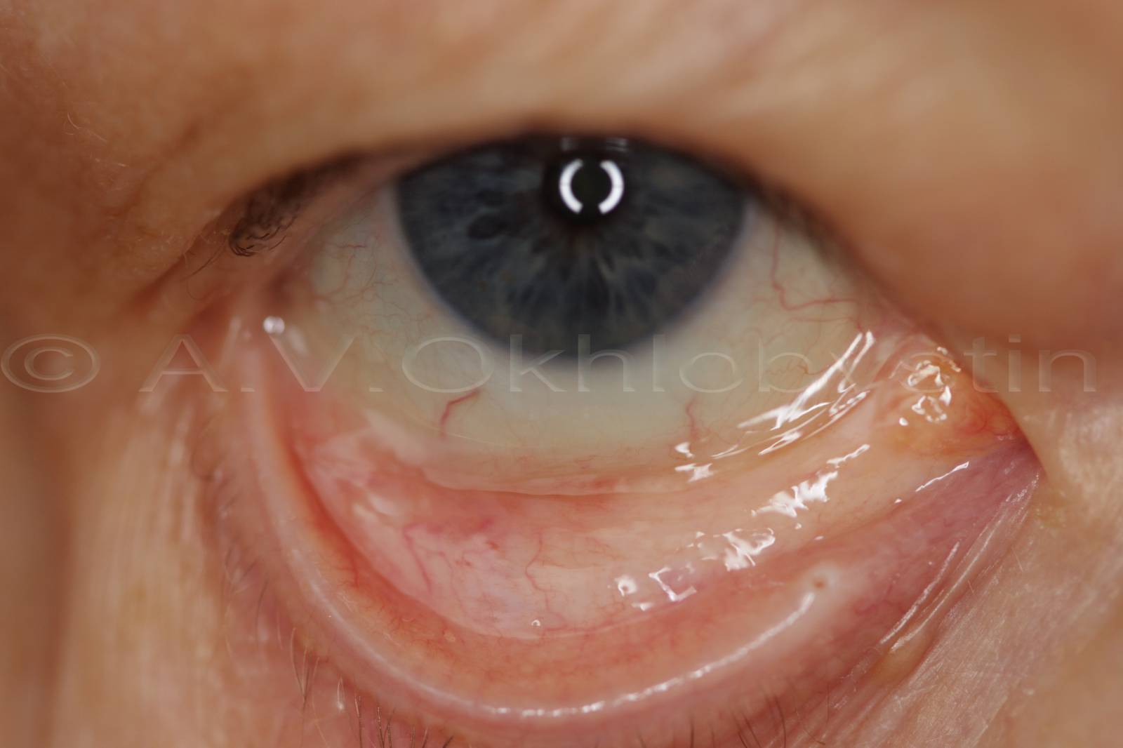
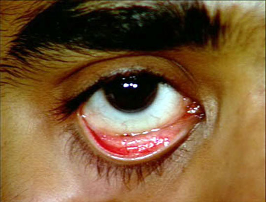
  10. 2016.05.11 identify the redness
  11. 2016.05.11 Iris Recognition Algorithms Comparison between Daugman algorithm and Hough transform on Matlab
  12. 2016.05.10 facerec framework
  13. 2016.05.09 OpenFace
  14. 2016.05.09 Face recognition with deep neural networks. http://cmusatyalab.github.io/openface/
  15. 2016.05.09 Facial Feature Tracking with SO-CLM
  16. 2016.05.09 gaze tracker
  17. 2016.04.12 TCPM (Tree Structured Parts Model) Tutorial
  18. 2016.03.09 Machine learning - → Professur Künstliche Intelligenz
  19. 2014.10.09 Generating the feature of GLOC
  20. 2014.09.30 Self-Tuning Spectral Clustering 64bit mex files
  21. 2013.08.23 Introduction to Machine Learning - 3/3
  22. 2013.08.23 Introduction to Machine Learning - 2/3
  23. 2013.08.23 Introduction to Machine Learning - 1/3
  24. 2013.08.21 Generative model VS Discriminative model
  25. 2013.08.21 What is the difference between a Generative and Discriminative Algorithm?
  26. 2013.08.21 discriminative vs. generative, classification vs. categorization
  27. 2013.06.26 Logistic Regression에 대한 간단한 설명
  28. 2013.06.12 Kristen Grauman - Visual Object Recognition and Image Search
  29. 2013.06.05 Kristen Grauman - Special Topics in Computer Vision, Spring 2010 1
  30. 2013.06.05 Kristen Grauman - Computer Vision Spring 2011

http://www.robots.ox.ac.uk/~vgg/publications/2015/Xie15/


This material is presented to ensure timely dissemination of scholarly and technical work. Copyright and all rights therein are retained by authors or by other copyright holders. All persons copying this information are expected to adhere to the terms and constraints invoked by each author's copyright. In most cases, these works may not be reposted without the explicit permission of the copyright holder.

Microscopy Cell Counting with Fully Convolutional Regression Networks

W. Xie, J. A. Noble, A. Zisserman
MICCAI 1st Workshop on Deep Learning in Medical Image Analysis, 2015
Download the publication : weidi15.pdf [2.1Mo]  
This paper concerns automated cell counting in microscopy images. The approach we take is to adapt Convolutional Neural Networks (CNNs) to regress a cell spatial density map across the image. This is applicable to situations where traditional single-cell segmentation based methods do not work well due to cell clumping or overlap. We make the following contributions: (i) we develop and compare architectures for two Fully Convolutional Regression Networks (FCRNs) for this task; (ii) since the networks are fully convolutional, they can predict a density map for an input image of arbitrary size, and we exploit this to improve efficiency at training time by training end-to-end on image patches; and (iii) we show that FCRNs trained entirely on synthetic data are able to give excellent predictions on real microscopy images without fine-tuning, and that the performance can be further improved by fine-tuning on the real images. We set a new state-of-the-art performance for cell counting on the standard synthetic image benchmarks and, as a side benefit, show the potential of the FCRNs for providing cell detections for overlapping cells.


BibTex reference:

@InProceedings{Xie15,
  author       = "Xie, W. and Noble, J.~A. and Zisserman, A.",
  title        = "Microscopy Cell Counting with Fully Convolutional Regression Networks",
  booktitle    = "MICCAI 1st Workshop on Deep Learning in Medical Image Analysis",
  year         = "2015",
}

Other publications in the database:


Posted by uniqueone
,
http://www.mathworks.com/matlabcentral/answers/105120-normalize-colors-under-different-lighting-conditions


I have done an outdoor experiment of a camera capturing images every 1 hour for color checker chart. I am trying to normalize each color so it looks the same through the day; as the color constancy is intensity independent.

I have tried several methods but the results were disappointing. Any ideas?

Thanks

---------------------------------------------------------------------------------------------

What methods did you try? Did you try cross channel cubic linear regression?

---------------------------------------------------------------------------------------------

I tried normalization for RGB channels user comprehensive color normalization

No, I haven't tried cross channel cubic linear regression.

---------------------------------------------------------------------------------------------

Try an equation like

newR = a0 + a1*R + a2*G + a3*B + a4*R*G + a5*R*B + a6*G*B + a7*R^2 + a8*G^2 + a9*B^2 + .....

See my attached seminar/tutorial on RGB-to-RGB color correction and RGB-to-LAB color calibration.


---------------------------------------------------------------------------------------------

Thank you, this method looks complicated whereas my application is simple. The only thing I want to do is to normalize a color throughout the day. For example, red through the day is shown as [black - brown - red - pink - white - pink - red - brown - black]. I want to stabilize this color to be red during the day. The data was taken from a CMOS imaging sensor.

---------------------------------------------------------------------------------------------

Attached is a super simple (dumb) way of doing it. Not too sophisticated and won't be as good in all situations but it might work for you. I would never use it though because it's not as accurate as we need for industrial use. It's more just for students to learn from.

  • crude_white_balancing.m
  •  

    ---------------------------------------------------------------------------------------------

    Thank you for this file. But this code converts colors to grey scale after correction. I want the result image to be colored

    ---------------------------------------------------------------------------------------------

    The result image is colored. Did you actually run it? With the onion image? And draw out a square over the yellowish onion? You'll see that the final corrected image is color. Try again. Post screenshots if you need to.

    ---------------------------------------------------------------------------------------------

    I don't know why you're processing each quadrilateral individually. Whatever happened to the image (lighting color shift, overall intensity shift, introduction of haze or whatever) most likely affected the whole image. I think if you processed each quadrilateral individually and then came up with 24 individual transforms, and then applied those individual transforms to the same area in the subject image, your subject image would look very choppy. So if your mid gray chip went from greenish in the morning to gray in the mid-day to bluish in the evening, those color shifts would apply to all chips. I've seen a lot of talks and posters at a lot of color conferences and talked to a lot of the worlds experts in color and I don't recall ever seeing anyone do what you want to do. There are situations in spectral estimation where you have a mixture of light (e.g. indoor fluorescent and outdoor daylight) both impinging on a scene and they want to estimate the percentage of light hitting different parts of the scene and the resultant spectrum so that you can get accurate color correction across the different illumination regions but you can't do that on something as small as a single X-rite Color Checker Chart. Anyway even if you did want to chop your scene up into 24 parts and have 24 transforms to fix up each of the 24 regions independently, you'd still have to do one of the methods I showed - either the more accurate regression, or the less accurate linear scaling - or something basically the same concept. You need a transform that take the R, G, and B and gives you a "fixed up" red. And another transform to fix green, and another transform to fix the blue.

    ---------------------------------------------------------------------------------------------

    Thank you very much.

    ---------------------------------------------------------------------------------------------


    Posted by uniqueone
    ,
    http://kr.mathworks.com/matlabcentral/answers/79147-how-to-color-correct-an-image-from-with-a-color-checker

    http_kr.mathworks.com_matlabcentral_answers_79147-how-to-colo.pdf


    We are developing an open source image analysis pipeline ( http://bit.ly/VyRFEr) for processing timelapse images of plants growing. Our lighting conditions vary dynamically throughout the day ( http://youtu.be/wMt5xtp9sH8) but we want to be able to automate removal of the background and then count things like green pixels between images of the same plant throughout the day despite the changing lighting. All the images have x-rite (equivalent) color checkers in them. I've looked through a lot of posts but I'm still a unclear on how we go about doing color (and brightness) correction to normalize the images so they are comparable. Am I wrong in assuming this is a relatively simple undertaking?

    Anyone have any working code, code samples or suggested reading to help me out?

    Thanks!

    Tim

    Sample images: Morning: http://phenocam.anu.edu.au/data/timestreams/Borevitz/_misc/sampleimages/morning.JPG

    Noon: http://phenocam.anu.edu.au/data/timestreams/Borevitz/_misc/sampleimages/noon.JPG

    -------------------------------------------------------------------------------------------

    Tim: I do this all the time, both in RGB color space, when we need color correction to a standard RGB image, and in XYZ color space, when we want calibrated color measurements. In theory it's simple, but the code and formulas are way too lengthy to share here. Basically for RGB-to-RGB correction, you make a model of your transform, say linear, quadratic, or cubic, with or without cross terms (RG, RB, R*B^2, etc.). Then you do a least squares model to get a model for Restimated, Gestimated, and Bestimated. Let's look at just the Red. You plug in the standard values for your 24 red chips (that's the "y"), and the values of R, G, B, RG, RB, GB, R^2G, etc. into the "tall" 24 by N matrix, and you do least squares to get the coefficients, alpha. Then repeat to get sets of coefficients beta, and gamma, for the estimated green and blue. Now, for any arbitrary RGB, you plug them into the three equations to get the estimated RGB as if that color was snapped at the same time and color temperature as your standard. If all you have are changes in intensity you probably don't need any cross terms, but if you have changes in the color of the illumination, then including cross terms will correct for that, though sometimes people do white balancing as a separate step before color correction. Here is some code I did to do really crude white balancing (actually too crude and simple for me to ever actually use but simple enough that people can understand it).

    I don't have any demo code to share with you - it's all too intricately wired into my projects. Someone on the imaging team at the Mathworks (I think it was Grant if I remember correctly) has a demo to do this. I think it was for the Computer Vision System Toolbox, but might have been for the Image Processing Toolbox. Call them and try to track it down. In the mean time try this: http://www.mathworks.com/matlabcentral/answers/?search_submit=answers&query=color+checker&term=color+checker

    --------------------------------------------------------------------------------------------

    Thanks, this is very helpful. Is there a quick and easy way to adjust white balance at least? Likewise for the color correction... if I don't need super good color correction but just want to clean up the lighting a bit without doing any high end color corrections is there a simple way to do this or do am I stuck figuring out how to do the full color correction or nothing?

    Thanks again.

    Tim

    ---------------------------------------------------------------------------------------------

    Did you ever get the demo from the Mathworks? If so, and they have it on their website, please post the URL.

    Here's a crude white balancing demo:

    % Does a crude white balancing by linearly scaling each color channel.
    clc;    % Clear the command window.
    close all;  % Close all figures (except those of imtool.)
    clear;  % Erase all existing variables.
    workspace;  % Make sure the workspace panel is showing.
    format longg;
    format compact;
    fontSize = 15;
    
    % Read in a standard MATLAB gray scale demo image.
    folder = fullfile(matlabroot, '\toolbox\images\imdemos');
    button = menu('Use which demo image?', 'onion', 'Kids');
    % Assign the proper filename.
    if button == 1
    	baseFileName = 'onion.png';
    elseif button == 2
    	baseFileName = 'kids.tif';
    end
    % Read in a standard MATLAB color demo image.
    folder = fullfile(matlabroot, '\toolbox\images\imdemos');
    % Get the full filename, with path prepended.
    fullFileName = fullfile(folder, baseFileName);
    if ~exist(fullFileName, 'file')
    	% Didn't find it there.  Check the search path for it.
    	fullFileName = baseFileName; % No path this time.
    	if ~exist(fullFileName, 'file')
    		% Still didn't find it.  Alert user.
    		errorMessage = sprintf('Error: %s does not exist.', fullFileName);
    		uiwait(warndlg(errorMessage));
    		return;
    	end
    end
    [rgbImage colorMap] = imread(fullFileName);
    % Get the dimensions of the image.  numberOfColorBands should be = 3.
    [rows columns numberOfColorBands] = size(rgbImage);
    % If it's an indexed image (such as Kids),  turn it into an rgbImage;
    if numberOfColorBands == 1
    	rgbImage = ind2rgb(rgbImage, colorMap); % Will be in the 0-1 range.
    	rgbImage = uint8(255*rgbImage); % Convert to the 0-255 range.
    end
    % Display the original color image full screen
    imshow(rgbImage);
    title('Double-click inside box to finish box', 'FontSize', fontSize);
    % Enlarge figure to full screen.
    set(gcf, 'units','normalized','outerposition', [0 0 1 1]);
    
    % Have user specify the area they want to define as neutral colored (white  or gray).
    promptMessage = sprintf('Drag out a box over the ROI you want to be neutral colored.\nDouble-click inside of it to finish it.');
    titleBarCaption = 'Continue?';
    button = questdlg(promptMessage, titleBarCaption, 'Draw', 'Cancel', 'Draw');
    if strcmpi(button, 'Cancel')
    	return;
    end
    hBox = imrect;
    roiPosition = wait(hBox);	% Wait for user to double-click
    roiPosition % Display in command window.
    % Get box coordinates so we can crop a portion out of the full sized image.
    xCoords = [roiPosition(1), roiPosition(1)+roiPosition(3), roiPosition(1)+roiPosition(3), roiPosition(1), roiPosition(1)];
    yCoords = [roiPosition(2), roiPosition(2), roiPosition(2)+roiPosition(4), roiPosition(2)+roiPosition(4), roiPosition(2)];
    croppingRectangle = roiPosition;
    
    % Display (shrink) the original color image in the upper left.
    subplot(2, 4, 1);
    imshow(rgbImage);
    title('Original Color Image', 'FontSize', fontSize);
    
    % Crop out the ROI.
    whitePortion = imcrop(rgbImage, croppingRectangle);
    subplot(2, 4, 5);
    imshow(whitePortion);
    caption = sprintf('ROI.\nWe will Define this to be "White"');
    title(caption, 'FontSize', fontSize);
    
    % Extract the individual red, green, and blue color channels.
    redChannel = whitePortion(:, :, 1);
    greenChannel = whitePortion(:, :, 2);
    blueChannel = whitePortion(:, :, 3);
    % Display the color channels.
    subplot(2, 4, 2);
    imshow(redChannel);
    title('Red Channel ROI', 'FontSize', fontSize);
    subplot(2, 4, 3);
    imshow(greenChannel);
    title('Green Channel ROI', 'FontSize', fontSize);
    subplot(2, 4, 4);
    imshow(blueChannel);
    title('Blue Channel ROI', 'FontSize', fontSize);
    
    % Get the means of each color channel
    meanR = mean2(redChannel);
    meanG = mean2(greenChannel);
    meanB = mean2(blueChannel);
    
    % Let's compute and display the histograms.
    [pixelCount grayLevels] = imhist(redChannel);
    subplot(2, 4, 6); 
    bar(pixelCount);
    grid on;
    caption = sprintf('Histogram of original Red ROI.\nMean Red = %.1f', meanR);
    title(caption, 'FontSize', fontSize);
    xlim([0 grayLevels(end)]); % Scale x axis manually.
    % Let's compute and display the histograms.
    [pixelCount grayLevels] = imhist(greenChannel);
    subplot(2, 4, 7); 
    bar(pixelCount);
    grid on;
    caption = sprintf('Histogram of original Green ROI.\nMean Green = %.1f', meanR);
    title(caption, 'FontSize', fontSize);
    xlim([0 grayLevels(end)]); % Scale x axis manually.
    % Let's compute and display the histograms.
    [pixelCount grayLevels] = imhist(blueChannel);
    subplot(2, 4, 8); 
    bar(pixelCount);
    grid on;
    caption = sprintf('Histogram of original Blue ROI.\nMean Blue = %.1f', meanR);
    title(caption, 'FontSize', fontSize);
    xlim([0 grayLevels(end)]); % Scale x axis manually.
    
    % specify the desired mean.
    desiredMean = mean([meanR, meanG, meanB])
    message = sprintf('Red mean = %.1f\nGreen mean = %.1f\nBlue mean = %.1f\nWe will make all of these means %.1f',...
    	meanR, meanG, meanB, desiredMean);
    uiwait(helpdlg(message));
    
    % Linearly scale the image in the cropped ROI.
    correctionFactorR = desiredMean / meanR;
    correctionFactorG = desiredMean / meanG;
    correctionFactorB = desiredMean / meanB;
    redChannel = uint8(single(redChannel) * correctionFactorR);
    greenChannel = uint8(single(greenChannel) * correctionFactorG);
    blueChannel = uint8(single(blueChannel) * correctionFactorB);
    % Recombine into an RGB image
    % Recombine separate color channels into a single, true color RGB image.
    correctedRgbImage = cat(3, redChannel, greenChannel, blueChannel);
    figure;
    % Display the original color image.
    subplot(2, 4, 5);
    imshow(correctedRgbImage);
    title('Color-Corrected ROI', 'FontSize', fontSize);
    % Enlarge figure to full screen.
    set(gcf, 'units','normalized','outerposition',[0 0 1 1]);
    
    % Display the color channels.
    subplot(2, 4, 2);
    imshow(redChannel);
    title('Corrected Red Channel ROI', 'FontSize', fontSize);
    subplot(2, 4, 3);
    imshow(greenChannel);
    title('Corrected Green Channel ROI', 'FontSize', fontSize);
    subplot(2, 4, 4);
    imshow(blueChannel);
    title('Corrected Blue Channel ROI', 'FontSize', fontSize);
    
    % Let's compute and display the histograms of the corrected image.
    [pixelCount grayLevels] = imhist(redChannel);
    subplot(2, 4, 6); 
    bar(pixelCount);
    grid on;
    caption = sprintf('Histogram of Corrected Red ROI.\nMean Red = %.1f', meanR);
    title(caption, 'FontSize', fontSize);
    xlim([0 grayLevels(end)]); % Scale x axis manually.
    % Let's compute and display the histograms.
    [pixelCount grayLevels] = imhist(greenChannel);
    subplot(2, 4, 7); 
    bar(pixelCount);
    grid on;
    caption = sprintf('Histogram of Corrected Green ROI.\nMean Green = %.1f', meanR);
    title(caption, 'FontSize', fontSize);
    xlim([0 grayLevels(end)]); % Scale x axis manually.
    % Let's compute and display the histograms.
    [pixelCount grayLevels] = imhist(blueChannel);
    subplot(2, 4, 8); 
    bar(pixelCount);
    grid on;
    caption = sprintf('Histogram of Corrected Blue ROI.\nMean Blue = %.1f', meanR);
    title(caption, 'FontSize', fontSize);
    xlim([0 grayLevels(end)]); % Scale x axis manually.
    
    % Get the means of the corrected ROI for each color channel.
    meanR = mean2(redChannel);
    meanG = mean2(greenChannel);
    meanB = mean2(blueChannel);
    correctedMean = mean([meanR, meanG, meanB])
    message = sprintf('Now, the\nCorrected Red mean = %.1f\nCorrected Green mean = %.1f\nCorrected Blue mean = %.1f\n(Differences are due to clipping.)\nWe now apply it to the whole image',...
    	meanR, meanG, meanB);
    uiwait(helpdlg(message));
    
    % Now correct the original image.
    % Extract the individual red, green, and blue color channels.
    redChannel = rgbImage(:, :, 1);
    greenChannel = rgbImage(:, :, 2);
    blueChannel = rgbImage(:, :, 3);
    % Linearly scale the full-sized color channel images
    redChannelC = uint8(single(redChannel) * correctionFactorR);
    greenChannelC = uint8(single(greenChannel) * correctionFactorG);
    blueChannelC = uint8(single(blueChannel) * correctionFactorB);
    
    % Recombine separate color channels into a single, true color RGB image.
    correctedRGBImage = cat(3, redChannelC, greenChannelC, blueChannelC);
    subplot(2, 4, 1);
    imshow(correctedRGBImage);
    title('Corrected Full-size Image', 'FontSize', fontSize);
    
    message = sprintf('Done with the demo.\nPlease flicker between the two figures');
    uiwait(helpdlg(message));
    Posted by uniqueone
    ,
    http://www.mathworks.com/matlabcentral/fileexchange/42548-consistent-imaging-with-consumer-cameras

    Consistent imaging with consumer cameras

    These set of scripts accompany the paper:

    Use of commercial-off-the-sgeld (COTS) digital cameras for scientific data acquisition and scene-specific color calibration

    by Akkaynak et al.

    The paper is currently in submission and the toolbox has been made available for testing in advance.

    code.zip


    Posted by uniqueone
    ,
    http://www.cs.ucf.edu/~bagci/teaching/mic16.html


    Special Topics CAP5937-Medical Image Computing (SPRING 2016)

    Assistant Professor  •  Computer Scientist  •  Imaging Expert  •   •  Home  •  Classes  •  CRCV  •  Research Blog  •  Publications  • 


    Instructor: Prof. Ulas Bagci    

    Class time: Monday/Wednesday 10.30-11.45 am
    Class location: HPA1 0106
    Office hours: Monday/Wednesday 3-5 pm

    COURSE GOALS: Imaging science is experiencing tremendous growth in the US. The New York Times recently ranked biomedical jobs as the number one fastest growing career field in the nation and listed bio-medical imaging as a primary reason for the growth. Biomedical imaging and its analysis are fundamental to understanding, visualizing, and quantifying medical images in clinical applications. With the help of automated and quantitative image analysis techniques, disease diagnosis will be easier/faster and more accurate, and leading to significant development in medicine in general. The goal of this course is to help students develop skills in computational radiology, radiological image analysis, and biomedical image processing fields. The following topics will be covered:

    • Basics of Radiological Image Modalities and their clinical use
    • Introduction to Medical Image Computing and Toolkits
    • Image Filtering, Enhancement, Noise Reduction, and Signal Processing
    • Medical Image Registration
    • Medical Image Segmentation
    • Medical Image Visualization
    • Machine Learning in Medical Imaging
    • Shape Modeling/Analysis of Medical Images

    PRE-REQUEST: Basic Probability/Statistics, a good working knowledge of any programming language (python, matlab, C/C++, or Java), Linear algebra, Vector calculus.

    GRADING:Assignments and mini projects should include explanatory/clear comments as well as a short report describing the approach, detailed analysis, and discussion/conclusion.

    • Programming assignments 30% (3 assignments, 10% each)
    • Midterm 20%
    • Project 50% (Presentation: 15%, Software/methods/results: 35%)

    RECOMMENDED BOOKS (optional)

    PROGRAMMING
    Students are enocouraged to use ITK/VTK programming libraries in implementation of the programming assignments and project.
    ITK is an open-source, cross-platform system that provides developers with an extensive suite of software tools for image analysis.
    The Visualization Toolkit (VTK) is an open-source, freely available software system for 3D computer graphics, image processing, and visualization. It consists of a C++ class library and several interpreted interface layers including Tcl/Tk, Java, and Python.

    Python and/or C/C++ can call functions of ITK/VTK easily. Matlab can be used for assignments as well.
    Following book (Python programming samples for computer viion tasks) is freely available.
    Python for Computer Vision

    COLLABORATION POLICY
    Collaboration on assignments is encouraged at the level of sharing ideas and technical conversation only. Please write your own code. Students are expected to abide by UCF Golden Rule.

    LECTURE NOTES

    PROGRAMMING ASSIGNMENTS

    POTENTIAL CLASS PROJECTS

    • Lung Lobe Segmentation from CT Scans (Use LOLA11 Segmentation Challenge Data Set)
    • Segmentation of Knee Images from MRI (Use SKI 2010 Data Set))
    • Multimodal Brain Tumor Segmentation (Use BraTS Data Set)
    • Automatic Lung Nodule (cancer) Detection (Use LUNA Data Set)
    • Automatically measure end-systolic and end-diastolic volumes in cardiac MRIs. (Use Kaggle Cardiac Data Set)
    • Head-Neck Auto Segmentation Challenge (Use MICCAI 2015 Segmentation Challange Data Set)
    • CAD of Dementia from Structural MRI (Use MICCAI 2014 Segmentation Challenge Data Set)
    • DTI Tractography Challenge (Use MICCAI 2014 Segmentation Challenge Data Set)
    • EMPIRE 2010 - Pulmonary Image Registration Challenge (http://empire10.isi.uu.nl/index.php, I have the team name and password for downloading the data set).
    • Digital Mammography DREAM challenge < LINK>
    • MACHINE LEARNING Challenge in medical imaging < LINK>)

    SELECTED PROJECTS FROM SPRING 2016 CLASS

    will be updated soon...

    Contact

    [Ulas Bagci in 2015]
    Ulas Bagci in 2009

    Name: Ulas Bagci
    Email:
    URL: http://www.cs.ucf.edu/~bagci
    Work number: (+1) 407-823-1047
    Fax number: (+1) 407-823-0594
    CRCV Assistant: Tonya LaPrarie
    Mailing address: Dr. Ulas Bagci
    Center for Research in Computer Vision (CRCV)
    4328 Scorpius Street, HEC 221, UCF

    Orlando, Florida 32816, USA.

    Last updated September, 2015 by Ulas Bagci.
    Posted by uniqueone
    ,
    Posted by uniqueone
    ,

    http://www.cockeyed.com/photos/bodies/heightweight.html


    BMI 예측 관련 프로젝트에서.

    Introduction

    This project implements the idea presented in the following paper:
    2013, Wen, Lingyun and Guo, Guodong
    A computational approach to body mass index prediction from face images
    The paper propsed that a person's body mass index (BMI) can be estimated from facial features without measuring the actual height and weight. A trained feature detector based on the active shape model (ASM) is used to extract points of interest on the face; then several facial features are calculated using the points. After features are computed on the dataset, a model is trained using machine learning approaches.

    Data

    The photos used in this project are crawled from a website containing photos with self reported height and weight information.

    (http://www.cockeyed.com/photos/bodies/heightweight.html)
    Posted by uniqueone
    ,

    http://www.mathworks.com/matlabcentral/answers/169911-cpp-file-in-matlab


    Hi,

    you will need to tell mex where to find the include files, and probably also the library files. Your call should look something like

    mex -I"C:\Program Files\opencv\include" Loadimage.cpp -l"C:\Program Files\opencv\lib" -Lopencv.lib
    

    Take a look at the doc for mex and there at the flags "-I", "-L", "-l".

    Titus

    Posted by uniqueone
    ,
    http://www.mathworks.com/matlabcentral/answers/10089-image-rotate


    Irot = imrotate(I,theta);
    Mrot = ~imrotate(true(size(I)),theta);
    Irot(Mrot&~imclearborder(Mrot)) = 255;
    
    %View 'er
    imtool(Irot)
    
    Posted by uniqueone
    ,

    redness = max(0, red - (blue + green) / 2);


    http://stackoverflow.com/questions/26135045/identify-the-redness-in-an-image-then-compare-with-the-other-image-using-matla

    I want to identify redness in the image and then compare that value with the redness in another image. I am quite new to Matlab and don't have image processing knowledge. However, I have been trying some random techniques to do this. Till now, I have used histograms of RGB channels of individual images and have also compared average numeric values of RGB channels in individual images. Unfortunately, I see almost similar results in both cases and cannot identify difference between less red and more red image.

    I randomly tried working with grayscale histograms as well but found it to be useless.

    P.S. I searched on this forum and tried to find a similar problem but i did not find anything that could help me. What I need is: a. Which technique could be used to check redness in images? b. How Matlab can me help there?

    %-------------------------------------------
    %For histograms of all 3 RGB channels in an image
    
    i = imread('<Path>\a7.png');
    imgr = i(:,:,1);
    imgg = i(:,:,2);
    imgb = i(:,:,3);
    histr = hist(imgr(:), bins);
    histg = hist(imgg(:), bins);
    histb = hist(imgb(:), bins);
    hfinal = [histr(:); histg(:); histb(:)];
    plot(bins, histr);
    
    
    %-------------------------------------------
    %To compare mean values of R channels of all images
    
    clear all; 
    %read all images in a sequence
    flist=dir('<Path>\*.png');
    
    for p = 1:length(flist)
        for q = 1 : 3
        fread = strcat('<Path>\',flist(p).name);
        im = imread(fread);
        meanim(p,q) = mean2(im(:,:,q));
        end
    end
    
    %disp(meanim);
    rm = meanim(:,1);
    frm = sum(rm(:));
    gm = meanim(:,2);
    fgm = sum(gm(:));
    bm = meanim(:,3);
    fbm = sum(bm(:));
    
    figure();
    set(0,'DefaultAxesColorOrder',[1 0 0;0 1 0;0 0 1]);
    pall = [rm(:), gm(:), bm(:)];
    plot(pall);
    title('Mean values of R, G and B in 12 images');
    leg1 = legend('Red','Green','Blue', ...
                    'Location','Best');
    print (gcf, '-dbmp', 'rgbchannels.bmp') 
    
    sm = sum(meanim);
    fsum = sum(sm(:));
    
    % disp(fsum);
    
    f2 = figure(2);
    set(f2, 'Name','Average Values');
    t = uitable('Parent', f2, 'Position', [20 20 520 380]);
    set(t, 'ColumnName', {'Average R', 'Average G', 'Average B'});
    set(t, 'Data', pall);
    print (gcf, '-dbmp', 'rgbtable.bmp') ;
    
    rgbratio = rm ./ fsum;
    disp(rgbratio);
    
    f3 = figure(3);
    aind = 1:6;
    hold on;
    subplot(1,2,1);
    plot(rgbratio(aind),'r+');
    title('Plot of anemic images - having more pallor');
    
    nind = 7:12;
    subplot(1,2,2);
    plot(rgbratio(nind),'b.');
    title('Plot of non anemic images - having less pallor');
    hold off;
    print (gcf, '-dbmp', 'anemicpics

    ------------------------------------------------------------------------------------------------------

    You can't assume the red channel is the same as the redness of a pixel by itself. A good estimate of redness of a pixel may be achieved by something like this:

    redness = max(0, red - (blue + green) / 2);

    Where red, green and blue are values of different RGB channels in the image. Once you calculated this value for an image, you can estimate the redness of the image by some approaches like averaging or histograms.

    'Digital Image Processing' 카테고리의 다른 글

    Using a Gray-Level Co-Occurrence Matrix (GLCM)  (0) 2017.02.03
    Embossing filter  (0) 2017.01.13
    Taking partial derivatives is easy in Matlab  (0) 2016.12.01
    Matlab Image Processing  (0) 2016.12.01
    Gabor Filter 이해하기  (0) 2016.10.17
    Posted by uniqueone
    ,
    https://github.com/Qingbao/iris


    iris

    Iris Recognition Algorithms Comparison between Daugman algorithm and Hough transform on Matlab.

    DESCRIPTION:

    Iris is one of the most important biometric approaches that can perform high confidence recognition. Iris contains rich and random Information. Most of commercial iris recognition systems are using the Daugman algorithm. The algorithms are using in this case from open sourse with modification, if you want to use the source code, please check the LICENSE.

    Daugman algorithm:

    image

    where I(x,y) is the eye image, r is the radius to searches over the image (x,y), G(r) is a Gaussian smoothing function. The algorithm starts to search from the pupil, in order to detect the changing of maximum pixel values (partial derivative).

    image

    image

    Hough transform:

    image

    The Hough transform is a feature extraction technique used in image analysis, computer vision, and digital image processing. where (xi, yi) are central coordinates, and r is the radius. Generally, and eye would be modeled by two circles, pupil and limbus (iris region), and two parabolas, upper and lower eyelids

    Starts to detect the eyelids form the horizontal direction, then detects the pupil and iris boundary by the vertical direction.

    image

    image

    NORMALIZATION AND FEATURE ENCODING:

    From circles to oblong block By using the 1D Log-Gabor filter. In order to extract 9600 bits iris code, the upper and lower eyelids will be processed as a 9600 bits mask during the encoding.

    image image image

    MATCHING:

    Hamming distance (HD): image where A and B are subjects to compare, which contains 20480=9600 template bits and 20480=9600 mask bits, respectively, in order to calculate by using XOR and AND boolean operators.

    Results:

    CASIA Iris Image Database(version 1.0) (http://biometrics.idealtest.org/dbDetailForUser.do?id=1): 756 iris images form 108 different subjects. High quality of images by using NIR camera.

    Resolution of 320*280.

    Totally, 756*755/2=285390 pairs of comparison for each algorithm, 2268 for intra-class comparison and 283 122 for inter-class comparison.

    EER:

    Daugman algorithm: 0.0157 Hough transform: 0.0500


    Posted by uniqueone
    ,

    facerec framework

    Computer Vision 2016. 5. 10. 09:45

    https://github.com/bytefish/facerec/wiki


    Home

    bytefish edited this page on Jan 10 2013 · 7 revisions

    facerec

    These wiki pages are not necessarily related to the facerec framework, but serve as a place to put interesting links, ideas, algorithms or implementations to. Feel free to extend the list, add new wiki pages or request new features in the issue tracker.

    Research

    Eye Tracking, Image Alignment and Head Pose Estimation

    Feature Extraction

    • Lior Wolf, Tal Hassner and Yaniv Taigman, Descriptor Based Methods in the Wild, Faces in Real-Life Images workshop at the European Conference on Computer Vision (ECCV), Oct 2008. (PDF Online available), (Matlab Code)
    • Ojansivu V & Heikkilä J (2008) Blur insensitive texture classification using local phase quantization. Proc. Image and Signal Processing (ICISP 2008), 5099:236-243. (PDF Online available), (Matlab Code)


    Posted by uniqueone
    ,

    OpenFace

    Computer Vision 2016. 5. 9. 16:41

    https://cmusatyalab.github.io/openface/


    OpenFace

    Free and open source face recognition with deep neural networks.


    News

    • 2016-01-19: OpenFace 0.2.0 released! See this blog post for more details.

    OpenFace is a Python and Torch implementation of face recognition with deep neural networks and is based on the CVPR 2015 paper FaceNet: A Unified Embedding for Face Recognition and Clustering by Florian Schroff, Dmitry Kalenichenko, and James Philbin at Google. Torch allows the network to be executed on a CPU or with CUDA.

    Crafted by Brandon Amos in Satya's research group at Carnegie Mellon University.


    This research was supported by the National Science Foundation (NSF) under grant number CNS-1518865. Additional support was provided by the Intel Corporation, Google, Vodafone, NVIDIA, and the Conklin Kistler family fund. Any opinions, findings, conclusions or recommendations expressed in this material are those of the authors and should not be attributed to their employers or funding sources.


    Isn't face recognition a solved problem?

    No! Accuracies from research papers have just begun to surpass human accuracies on some benchmarks. The accuracies of open source face recognition systems lag behind the state-of-the-art. See our accuracy comparisons on the famous LFW benchmark.


    Please use responsibly!

    We do not support the use of this project in applications that violate privacy and security. We are using this to help cognitively impaired users sense and understand the world around them.


    Overview

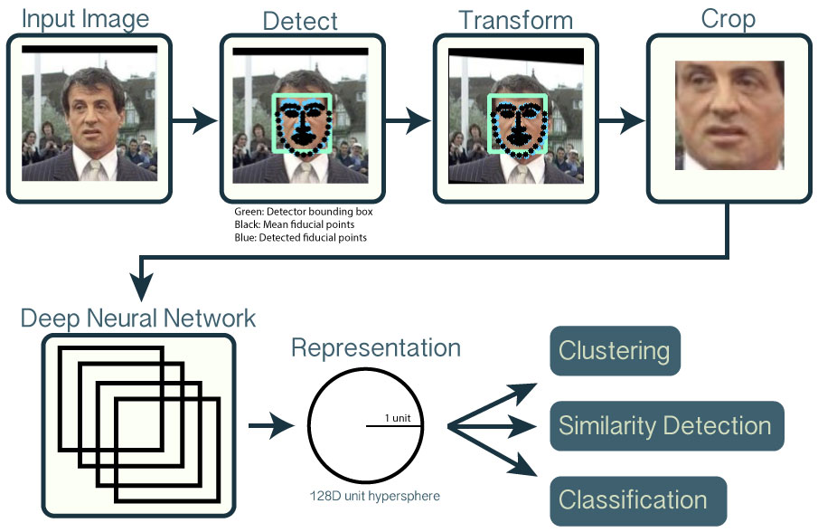
    The following overview shows the workflow for a single input image of Sylvestor Stallone from the publicly available LFW dataset.

    1. Detect faces with a pre-trained models from dlib or OpenCV.
    2. Transform the face for the neural network. This repository uses dlib's real-time pose estimation with OpenCV's affine transformation to try to make the eyes and bottom lip appear in the same location on each image.
    3. Use a deep neural network to represent (or embed) the face on a 128-dimensional unit hypersphere. The embedding is a generic representation for anybody's face. Unlike other face representations, this embedding has the nice property that a larger distance between two face embeddings means that the faces are likely not of the same person. This property makes clustering, similarity detection, and classification tasks easier than other face recognition techniques where the Euclidean distance between features is not meaningful.
    4. Apply your favorite clustering or classification techniques to the features to complete your recognition task. See below for our examples for classification and similarity detection, including an online web demo.

    News

    Blogosphere

    Projects using OpenFace

    Citations

    The following is a BibTeX and plaintext reference for the OpenFace GitHub repository. The reference may change in the future. The BibTeX entry requires the url LaTeX package.

    @misc{amos2016openface,
        title        = {{OpenFace: Face Recognition with Deep Neural Networks}},
        author       = {Amos, Brandon and Ludwiczuk, Bartosz and Harkes, Jan and
                        Pillai, Padmanabhan and Elgazzar, Khalid and Satyanarayanan, Mahadev},
        howpublished = {\url{http://github.com/cmusatyalab/openface}},
        note         = {Accessed: 2016-01-11}
    }
    
    Brandon Amos, Bartosz Ludwiczuk, Jan Harkes, Padmanabhan Pillai,
    Khalid Elgazzar, and Mahadev Satyanarayanan.
    OpenFace: Face Recognition with Deep Neural Networks.
    http://github.com/cmusatyalab/openface.
    Accessed: 2016-01-11
    

    Acknowledgements

    Licensing

    Unless otherwise stated, the source code and trained Torch and Python model files are copyright Carnegie Mellon University and licensed under the Apache 2.0 License. Portions from the following third party sources have been modified and are included in this repository. These portions are noted in the source files and are copyright their respective authors with the licenses listed.

    Project Modified License
    Atcold/torch-TripletEmbedding No MIT
    facebook/fbnn Yes BSD

    Posted by uniqueone
    ,
    https://github.com/cmusatyalab/openfaceOpenFace • Build Status Release License Gitter

    Free and open source face recognition with deep neural networks.


    This research was supported by the National Science Foundation (NSF) under grant number CNS-1518865. Additional support was provided by the Intel Corporation, Google, Vodafone, NVIDIA, and the Conklin Kistler family fund. Any opinions, findings, conclusions or recommendations expressed in this material are those of the authors and should not be attributed to their employers or funding sources.

    What's in this repository?

    Citations

    The following is a BibTeX and plaintext reference for the OpenFace GitHub repository. The reference may change in the future. The BibTeX entry requires the url LaTeX package.

    @misc{amos2016openface,
        title        = {{OpenFace: Face Recognition with Deep Neural Networks}},
        author       = {Amos, Brandon and Ludwiczuk, Bartosz and Harkes, Jan and
                        Pillai, Padmanabhan and Elgazzar, Khalid and Satyanarayanan, Mahadev},
        howpublished = {\url{http://github.com/cmusatyalab/openface}},
        note         = {Accessed: 2016-01-11}
    }
    
    Brandon Amos, Bartosz Ludwiczuk, Jan Harkes, Padmanabhan Pillai,
    Khalid Elgazzar, and Mahadev Satyanarayanan.
    OpenFace: Face Recognition with Deep Neural Networks.
    http://github.com/cmusatyalab/openface.
    Accessed: 2016-01-11
    

    Licensing

    Unless otherwise stated, the source code and trained Torch and Python model files are copyright Carnegie Mellon University and licensed under the Apache 2.0 License. Portions from the following third party sources have been modified and are included in this repository. These portions are noted in the source files and are copyright their respective authors with the licenses listed.

    Project Modified License
    Atcold/torch-TripletEmbedding No MIT
    facebook/fbnn Yes BSD


    'Computer Vision' 카테고리의 다른 글

    facerec framework  (0) 2016.05.10
    OpenFace  (0) 2016.05.09
    Facial Feature Tracking with SO-CLM  (0) 2016.05.09
    gaze tracker  (0) 2016.05.09
    TCPM (Tree Structured Parts Model) Tutorial  (0) 2016.04.12
    Posted by uniqueone
    ,
    http://kylezheng.org/facial-feature-mobile-device/


    Facial Feature Tracking with SO-CLM

    Facial Feature Detection and Tracking with Approximated Structured Output Learning based Constrained Local Model

    Shuai Zheng1  Paul Sturgess Philip H. S. Torr1

    1Brookes Vision Group, (Now Torr-Vision at University of Oxford)

    Abstract

    An approximated structured output learning approach is developed to learn the appearance model from CLM overtime on low-powered portable devices, such as iPad 2, iPhon 4S, Galaxy S2.

    Facial feature detection and tracking are very important in many applications such as face recognition, and face animation.

    comparisondifferent1


    What has been done

    Existing facial feature detectors like tree-structured SVM, Constrained Local Model (CLMs) achieve the state-of-the-art accuracy performance in many benchmarks (e.g. CMU MultiPIE, BioID etc.). However, when it comes to the low-powered device application, the trade-off among accuracy, speed and memory cost becomes apparently the main concern in the facial feature detection related application.

    ipad3

    How to make facial feature detection efficient in speed and memory

    There are two ways to address the speeding up problem. One is to use GPU(e.g. CUDA), and parallel computing (e.g. OpenMP) techniques to speed up the existing algorithms (e.g. AAM, CLM etc). Another is to improve the steps inside existing algorithms, or let’s say developing a new algorithm. In this paper, we explored how to speed up the facial feature detection with an approach called approximate structured output learning for constrained local model.

    converpagenew

    What we did

    Within this paper we examine the learning of the appearance model in Constrained Local Models (CLM) technique. We have two contributions: firstly we examine an approximate method for doing structured learning, which jointly learns all the appearances of the landmarks. Even though this method has no guarantee of optimality we find it performs better than training the appearance models independently. This also allows for efficiently online learning of a particular instance of a face. Secondly we use a binary approximation of our learnt model that when combined with binary features, leads to efficient inference at runtime using bitwise AND operations. We quantify the generalization performance of our approximate SO-CLM, by training the model parameters on a single dataset, and testing on a total of five unseen benchmarks.

    The speed at runtime is demonstrated on the ipad2 platform. Our results clearly show that our proposed system runs in real-time, yet still performs at state-of-the-art levels of accuracy.

    Publication

    [1] S. Zheng, P. Sturgess, and P. Torr, “Approximate Structured Output Learning for Constrained Local Models with Application to Real-time Facial Feature Detection and Tracking on Low-power Devices”, IEEE Conference on Automatic Face and Gesture Recognition (AFGR) , 2013.[[pdf][bib][poster][ppt][ResultsFig][IEEExplore]

    Software

    [1] Demo Program. [7.2M Win64ExcutableProgram][Win32][Linux][Mac]

    FAQ: you can get the detection results by type “BrookesFaceTracker.exe gaga.png”, you can get demo by type”BrookesFaceTracker.exe”.

    Data

    Frontal Facial landmark Annotation Dataset [link]

    Acknowledgement

    This project is supported by EPSRC EP/I001107/1.


    Related Links

    [1] S. Hare, A. Saffari, and P. Torr, “Efficient Online Structured Output Learning for Keypoint-based Object Tracking“, CVPR, 2012.[paper&C++code]

    [2] X. Zhu, D. Ramanan, “Face Detection, pose estimation and landmark localization in the wild“, CVPR, 2012. [project]

    [3] Struct SVM. [project]

    [4] Struct SVM in Matlab.[Project]

    [5] Flandmark. [project]

    [6] CI2CV. [Website]

    [7] CLM-Wlid [Website].

    [8] FacePlusPlus[Website]

    Data Links

    [1] BioID http://www.bioid.com/index.php?q=downloads/software/bioid-face-database.html

    [2] CMU MultiPie http://www.flintbox.com/public/project/4742/

    [3] XM2VTS http://www.ee.surrey.ac.uk/CVSSP/xm2vtsdb/

    [4] LFPW http://www.kbvt.com/LFPW/

    [5] Talking face http://www-prima.inrialpes.fr/FGnet/data/01-TalkingFace/talking_face.html

    [6]300 Faces in-the-wild [i-Bug webiste]

    Posted by uniqueone
    ,

    gaze tracker

    Computer Vision 2016. 5. 9. 16:04

    https://github.com/trishume/eyeLike


    eyeLike

    An OpenCV based webcam gaze tracker based on a simple image gradient-based eye center algorithm by Fabian Timm.

    DISCLAIMER

    This does not track gaze yet. It is basically just a developer reference implementation of Fabian Timm's algorithm that shows some debugging windows with points on your pupils.

    If you want cheap gaze tracking and don't mind hardware check out The Eye Tribe. If you want webcam-based eye tracking contact Xlabs or use their chrome plugin and SDK. If you're looking for open source your only real bet is Pupil but that requires an expensive hardware headset.

    Status

    The eye center tracking works well but I don't have a reference point like eye corner yet so it can't actually track where the user is looking.

    If anyone with more experience than me has ideas on how to effectively track a reference point or head pose so that the gaze point on the screen can be calculated contact me.

    Building

    CMake is required to build eyeLike.

    OSX or Linux with Make

    # do things in the build directory so that we don't clog up the main directory
    mkdir build
    cd build
    cmake ../
    make
    ./bin/eyeLike # the executable file

    On OSX with XCode

    mkdir build
    ./cmakeBuild.sh

    then open the XCode project in the build folder and run from there.

    On Windows

    There is some way to use CMake on Windows but I am not familiar with it.

    Blog Article:

    Paper:

    Timm and Barth. Accurate eye centre localisation by means of gradients. In Proceedings of the Int. Conference on Computer Theory and Applications (VISAPP), volume 1, pages 125-130, Algarve, Portugal, 2011. INSTICC.

    (also see youtube video at http://www.youtube.com/watch?feature=player_embedded&v=aGmGyFLQAFM)

    eyeLike-master.zip

    Posted by uniqueone
    ,
    https://github.com/jhlddm/TSPM


    TCPM (Tree Structured Parts Model) Tutorial

    Table of Contents


    Copyright

    This code is entirely based on the published code [1]. This document is a tutorial that instructs how to exploit this code with the mixture of models in the original code replaced with yours.

    [1] Xiangxin Zhu, Deva Ramanan. Face detection, pose estimation, and landmark localization in the wild. Computer Vision and Pattern Recognition (CVPR) Providence, Rhode Island, June 2012.

    Design a mixture of models

    We use a mixture of models for face detection. Let's first look into the original model implemented in the code. As for the original mixture of models, total of 13 models form a mixture. Model 1 to 3 have the same tree structure, and are of purpose of detecting human faces which are heading left. Model 4 to 10, in sequence, have the same tree structure, and these 7 are for detecting the frontal faces. The remaining 3 (model 11 to 13) have the same tree structure, and are for detecting the faces heading right.

    For better understanding, structure of the model 7 is constructed like below:

    Model 7: Frontal facial model

    Note that there are two kinds of labeling (numbering) systems. One is annotation order and the other is tree order. Annotation order is the ordering system under which the annotations (coordinates of landmark points) on the training images were made, while tree order is of the actual tree structure of a model used on the score evaluation stage.

    If you want to use a new facial model, follow the next steps.

    1. Construct a mixture of models. Decide how many models the mixture consists of.
    2. Design a tree structure which fit to the human faces for each model.
    3. Give labels to nodes of trees. As mentioned earlier, each node should be labeled with two numbers, one for annotation ordering system, and the other for tree ordering system.

    • Annotation order: If you have annotations within the training data, then you have to follow the labeling order of those annotations.
    • Tree order: Be aware that the id number of parent nodes should be larger than their children's.

    For example, simpler model might be like:

    Simpler model example

    The following material of this document is based on a mixture of models which consists of 3 models. Each of three models corresponds to viewpoints of 30, 0, -30 degree, respectively. And all the models have the same tree structure as shown above.

    Prepare dataset

    For training set, we need data of following files to be prepared:

    • Image files that include the human faces which we aim to detect.
    • Annotation files on images that include the coordinate values of landmark points (same as the center of parts in the models)

    For each of all the image files, there should be an annotation file named "[Image file name]_lb.mat" in the certain directory for annotation files. These are .mat files, where the coordinate values of landmark points are stored using a matrix variable named "pts". As for our simple model, size of the matrix "pts" is 15 by 2, cause we have 15 landmark points per an image. The first column refers to the x values of landmark points, and the second column refers to the y values, and each of 15 rows corresponds to each landmark point.

    The training data might be structured like:

    [ Image files ]
    *image_dir*/*image_name_1.jpg*
    ...
    *image_dir*/*image_name_n.jpg*
    
    [ Annotation files ]
    *anno_dir*/*image_name_1_lb.mat*
    ...
    *anno_dir*/*image_name_n_lb.mat*
    

    Edit multipie_init.m

    As the first step of change in codes, open "multipie_init.m" file located at the project root directory, and modify as follows.

    First of all, see the following part of the code.

    opts.viewpoint = 90:-15:-90;
    opts.partpoolsize = 39+68+39;
    

    opts.viewpoint is a list consisting of the viewpoint angles which the objects face towards. As for the original setting above, for example, it means that we aim to detect the human faces each of which is heading at 90 degree, 75 degree, ..., -90 degree respectively. (zero degree corresponds to the frontal view.)

    opts.partpoolsize is a sum over the number of parts of every different model. In the original setting, we have total of 3 different models for detecting the left, front, and right side of faces. These three models are composed of 39, 68, and 39 parts respectively. Thus we have the value of 39+68+39 in result.

    Change these two properly to work well with our model. Then the code above should be modified to be like:

    opts.viewpoint = [30, 0, -30];
    opts. partpoolsize = 15;
    

    And then, we specify mixture of models concretly. We have three models in our mixture of models, so what we have to do in this section is to define opts.mixture(1), opts.mixture(2), and opts.mixture(3) which correspond to our three models.

    Let's define a opts.mixture(1) first.

    At first, poolid should be a list of integer from 1 to 15, because every single model of our mixture has 15 parts.

    Next, the variable I and J define a transformation relation between the annotation and tree order labels. Let I have a array of integer range from 1 to the number of parts. And then, take a close look at J. The k'th number in array J, say nk, means that the node labeled with k in tree order is labeled with nk in annotation order.

    S in the next line should be modified to be the array consisting of ones that takes the number of parts as it's length.

    Using the variables defined above, we set the anno2treeorder to represent the transformation matrix from annotation to tree order. Just replace the 4th, and 5th argument of the sparse() function with the number of parts.

    Finally, pa specifies the id number of parent of each nodes. Note that you should follow the tree order in refering to a node here.

    As a result, the original codes might be changed as follows:

    % Global mixture 1 to 3, left, frontal, and right face
    opts.mixture(1).poolid = 1:15;
    I = 1:15;
    J = [9 10 11 8 7 3 2 1 6 5 4 12 13 14 15];
    S = ones(1,15);
    opts.mixture(1).anno2treeorder = full(sparse(I,J,S,15,15)); % label transformation
    opts.mixture(1).pa = [0 1 1 1 4 5 6 7 5 9 10 1 12 12 12];
    
    opts.mixture(2) = opts.mixture(1);
    opts.mixture(3) = opts.mixture(1);
    

    Edit multipie_data.m

    This "multipie_data.m" file does the data preparation work.

    First, define what images in our dataset will be used for training set, and what images for test set. Modify the lists trainlist and testlist properly based on the prepared dataset.

    Next, set the pathes where the image and annotation in the dataset are located. multipiedir is a path for image files, and annodir is a path for annotation files.

    Edit multipie.mat

    This .mat file includes a struct variable named multipie which includes the name of the image files classified by the models in our mixture. You may consult the "make_multipie_info" script in tools/ directory to make your own multipie variable more easily.

    Run multipie_main.m

    1. Run "compile.m" file first.
    2. Run "multipie_main" file. This script trains the model using the prepared dataset, evaluate the trained model, and even shows the result graphically.


    'Computer Vision' 카테고리의 다른 글

    Facial Feature Tracking with SO-CLM  (0) 2016.05.09
    gaze tracker  (0) 2016.05.09
    Generating the feature of GLOC  (0) 2014.10.09
    Self-Tuning Spectral Clustering 64bit mex files  (0) 2014.09.30
    Logistic Regression에 대한 간단한 설명  (0) 2013.06.26
    Posted by uniqueone
    ,

     https://www.tu-chemnitz.de/informatik/KI/edu/ml/

    Machine learning

    Content

    The course will present an introduction to the research field of Machine Learning, including Supervised Learning, Unsupervised Learning and Reinforcement Learning methods. The different algorithms presented during the lectures will be studied in more details during the exercises, through implementations in Python. Previous knowledge of Python is a plus.

    The plan of the course is:

    1. Supervised Learning
      1. Linear classification and regression
      2. Learning Theory
      3. Neural Networks
      4. Support vector machines
    2. Unsupervised Learning
      1. Clustering
      2. PCA, LDA
      3. Deep learning
    3. Reinforcement Learning
      1. Formal definition of the RL-Problem
      2. Dynamic Programming
      3. Monte Carlo Methods
      4. Temporal Difference Learning (TD)


    General Information

    Prerequisites: Modules in Mathematics I to IV, basic knowledge in Python.

    Exam: oral examination (20 minutes), 5 credit points.

    Contact: julien dot vitay at informatik dot tu-chemnitz dot de.

    Exam dates in 2016: 16.02, 22.02, 23.02, 29.02, 01.03, 02.03 and 03.03.

    Registration closed! Deregistration is only possible until one week prior to the appointment. No rescheduling possible.

    Exam location: in my office 1/348.

    Surya Narayana Varma Ruddaraju: empty your mailbox! Your exam is on 02.03 at 10:45.

    Literature

    Slides for the lectures

    Chapter 01 - Introduction
    Chapter 02 - Linear learning machines
    Chapter 03 - Learning theory
    Chapter 04 - Neural networks
    Chapter 05 - Support-vector machines
    Chapter 06 - Clustering, dimensionality reduction
    Chapter 07 - Deep learning.
    Chapter 08 - Reinforcement Learning.

    Exercises and solutions

    Exercise 01 - Introduction to Python and NumPy. Text - Data - Solution.
    Exercise 02 - Linear classification. Text - Data - Solution.
    Exercise 03 - Cross-validation. Text - Data - Solution.
    Exercise 04 - Multi-layer perceptron. Text - Data - Solution.
    Exercise 05 - Multi-layer perceptron on the MNIST dataset. Text - Data - Solution.
    Exercise 06 - Support-vector machines. Text - Data.
    Exercise 07 - K-means. Text - Data - Solution.
    Exercise 08 - PCA. Text - Data.
    Exercise 09 - Reinforcement learning. Text - Solution.

    ------------------------------------------------------------------------------


    exercise1-solution.zip


    exercise1.pdf


    exercise1.zip


    exercise2-solution.zip


    exercise2.pdf


    exercise2.zip


    exercise3-solution.zip


    exercise3.pdf


    exercise3.zip


    exercise4-solution.zip


    exercise4.pdf


    exercise4.zip


    exercise5.pdf


    exercise6.pdf


    exercise6.zip


    exercise7-solution.zip


    exercise7.pdf


    exercise7.zip


    exercise8.pdf


    exercise9-solution.zip


    exercise9.pdf


    ML01.pdf


    ML02.pdf


    ML03.pdf


    ML04.pdf


    ML05.pdf


    ML06.pdf


    ML08.pdf


    Posted by uniqueone
    ,

    Augmenting CRFs with Boltzmann Machine Shape Priors for Image Labeling.
    http://vis-www.cs.umass.edu/GLOC/

    http://vis-www.cs.umass.edu/lfw/part_labels/

    The authors' feature Code:
    The following code is used to generate the features.

    [gloc_features.zip] (md5sum 4bab12e8bea70ada9a7024f9166f9109)

    However, it produces some error in my MS VS2010 on Windows 7 (64-bit).

    I modified itgenerate_features1.cpp

    It needs OpenCV lib and it needs 'Command Argument' as follows.


    parts_all.txt

    LABClusterFile

    G:\Research\faceSeg\database\LFW\lfw_unfunneled\lfw_unfunneled

    G:\Research\faceSeg\database\LFW\lfw_superpixels_fine

    G:\Research\faceSeg\database\LFW\lfw_unfunneled\parts_lfw_unfunneled_spseg_features

    G:\Research\faceSeg\database\LFW\lfw_unfunneled\parts_lfw_unfunneled_gt_images

    G:\Research\faceSeg\database\LFW\lfw_unfunneled\parts_lfw_unfunneled_gt_images_generate

    G:\Research\faceSeg\database\LFW\lfw_unfunneled\parts_lfw_unfunneled_superpixels_mat

    G:\Research\faceSeg\database\LFW\lfw_unfunneled\parts_lfw_unfunneled_tex

    G:\Research\faceSeg\database\LFW\lfw_unfunneled\parts_lfw_unfunneled_pb


    1. parts_all.txt: File List. Provided in the authors homepage.

    2. LABClusterFile: LAB Cluster File. It will be created. Just type in 'Command Argument'

    3. G:\Research\faceSeg\database\LFW\lfw_unfunneled\lfw_unfunneled: LFW image Directory

    4. G:\Research\faceSeg\database\LFW\lfw_superpixels_fine: Superpixel Directory. The folder of Superpixel PPM files.

    5. G:\Research\faceSeg\database\LFW\lfw_unfunneled\parts_lfw_unfunneled_spseg_features: Features Directory. Feature will be save in this directory. 

     6. G:\Research\faceSeg\database\LFW\lfw_unfunneled\parts_lfw_unfunneled_gt_images:  Face and hair Ground Truth PPM files directory.

    7. G:\Research\faceSeg\database\LFW\lfw_unfunneled\parts_lfw_unfunneled_gt_images_generate: will be generated.

    8. G:\Research\faceSeg\database\LFW\lfw_unfunneled\parts_lfw_unfunneled_superpixels_mat: Superpixel label files in '.dat' extension.

    9. G:\Research\faceSeg\database\LFW\lfw_unfunneled\parts_lfw_unfunneled_tex: texture files generated from running 'generate_textures.m'.

    10. G:\Research\faceSeg\database\LFW\lfw_unfunneled\parts_lfw_unfunneled_pb: boundary infor. files generated from running 'generate_PB.m'.


    Posted by uniqueone
    ,

    Self-Tuning Spectral Clustering

    -->http://www.vision.caltech.edu/lihi/Demos/SelfTuningClustering.html


    I tried to operate the ZPclustering code, but it shows me some errors as follows, and it is because I'm using 64-bit matlab (on Windows 7).

    ------------------------------------------

    >> test_segimage
    Building affinity matrix took 0.063324 second

    Error using dist2aff
    Function "mxGetIr_700" is obsolete.
    (64-bit mex files using sparse matrices must be rebuilt with the "-largeArrayDims" option.  See the R2006b release notes for more details.)

    Error in segment_image (line 65)
        tic; W = dist2aff(D,SS); ttt = toc;

    Error in test_segimage (line 11)
    [mask] = segment_image(IM,R,G1,'SS','KM',0.1);

    ------------------------------------------

    I modified the mex files 

    dist2aff.cppevrot.cppscale_dist.cppzero_diag.cpp

    And, I typed like follows in matlab command window:

    >> mex -O -largeArrayDims -c dist2aff.cpp
    >> mex -O -largeArrayDims -c scale_dist.cpp
    >> mex -O -largeArrayDims -c zero_diag.cpp
    >> mex -O -largeArrayDims -c evrot.cpp


    >> mex -O -largeArrayDims  dist2aff.obj
    >> mex -O -largeArrayDims   scale_dist.obj
    >> mex -O -largeArrayDims  zero_diag.obj
    >> mex -O -largeArrayDims evrot.obj


    After that, it opertes well.

    Posted by uniqueone
    ,

    http://cs.brown.edu/courses/archive/2006-2007/cs195-5/calendar.html

    IntroML.vol3.egg


    Syllabus, lecture slides, homework assignments and solutions, etc.

    Note: All handouts and lecture slides are in PDF format. Any scheduling information posted for future dates should be treated as tentative.

    Abbreviation: DHS - Duda et al.; PRML - Bishop's new book; HTF - Hastie et al.; NNPR - Bishop's older book; MK - MacKay.

    • Wed 9/6/06
      • General introduction: goals of machine learning, examples, administrivia.
      • Lecture 1


    • Fri 9/8/06 Note: change of location to CIT 368


    • Mon 9/11/06 Note: change of location to CIT 368

      • Optimal regression function
      • statistical regression models, likelihood and log-likelihood
      • Maximum likelihood estimation
      • Lecture 3
      • Notes (derivations etc.)
      • Recommended reading: DHS A.2 (appendix), HTF 3.1-3.3, PRML 3.1.


    • Wed 9/13/06


    • Fri 9/15/06 In Lubrano, our new home

      • Introduction to classfication
      • A more detailed look at multivariate Gaussians
      • Linear Discriminant Analysis
      • Lecture 5
      • Another useful short summary by Sam Roweis, on Gaussian identities.
      • Recommended reading: NNPR 3.6; DHS A.4, A.5; HTF 4.1-4.3; PRML 2.3, 4.1, Appendices B,C.


    • Mon 9/18/06


    • Wed 9/20/06

      • Decision theory: Bayes rule, optimal classification.
      • Generative models for classification
      • Discriminant functions
      • Lecture 7
      • Recommended reading: PRML 1.5.1, HTF 2.4, DHS 2.1-2.7.


    • Fri 9/22/06

      • Estimation theory
      • Bias-variance tradeoff
      • Lecture 8


    • Mon 9/25/06

      • Bias-variance tradeoff and model complexity
      • Naive Bayes classifier
      • Applications in document classification
      • Bayesian estimation, MAP
      • Lecture 9
      • Recommended reading: PRML 2.2.2, 3.2; HTF 7.2-7.3; DHS 9.3; NNPR 9.1.


    • Wed 9/27/06


    • Fri 9/29/06

      • Logistic regression
      • Lecture 11
      • Recommended reading: NNPR 3.1.3, PRML 4.3.2-4.3.4.


    • Mon 10/2/06

      • Logistic regression: gradient ascent algorithms.
      • Computational issues, convergence.
      • Overfitting and regularization.
      • Lecture 12
      • Recommended reading: TBD.


    • Wed 10/4/06


    • Fri 10/6/06

      • Regularized regression: ridge regression and lasso.
      • Survey of what we have learned so far.
      • Large margin discriminative classifiers.
      • Lecture 14
      • Recommended reading: PRML 3.1.4, NNPR 9.2, HTF 3.4.


    • Mon 10/9/06

      • No class - Columbus Day


    • Wed 10/11/06

      • Support Vector Machines.
      • Problem Set 2 due.
      • Lecture 15
      • Recommended reading: PRML 7.1; HTF 12.2-12.3; DHS 5.11.
      • C. Burges, SVM tutorial.


    • Fri 10/13/06

      • Guest lecture: optimization.


    • Mon 10/16/06


    • Wed 10/18/06

      • Guest lecture: unsupervised and reinforcement learning in robotics.


    • Fri 10/20/06

      • Support Vector Machines: non-separable case, the kernel trick.
      • Lecture 16
      • Recommended reading: PRML 7.1; HTF 12.2-12.3; DHS 5.11.


    • Mon 10/23/06

      • Non-parametric methods; nearest-neighbor methods.
      • Lecture 17


    • Wed 10/25/06


    • Fri 10/27/06 CIT 367


    • Mon 10/30/06


    • Wed 11/1/06

      • The EM algorithm for Gaussian mixtures.
      • Recommended reading: PRML Chapter 9; HTF 8.5; DHS 3.9; NNPR 2.6.
      • Lecture 20


    • Fri 11/3/06

      • General view of EM; model selection.
      • Recommended reading: PRML Chapter 9; HTF 8.5; DHS 3.9; NNPR 2.6.
      • Lecture 21


    • Mon 11/6/06


    • Wed 11/8/06

      • Unsupervised learning, clustering, K-means.
      • Recommended reading: PRML 9.1, HTF 14.3
      • Lecture 23


    • Fri 11/10/06

    • Mon 11/13/06


    • Wed 11/15/06

      • Dimensionality reduction; Principal Component Analysis
      • Recommended reading: HTF 14.5, NNPR 8.6, PRML 12.1
      • Lecture 26


    • Fri 11/17/06


    • Mon 11/20/06


    • Wed 11/22/06

      • AdaBoost
      • Recommended reading: PRML 14.3, HTF 10.1-10.6
      • Lecture 29
      • Problem Set 5 due
      • Project proposals due (200-level)


    • Fri 11/24/06

      • No class - Thanksgiving recess


    • Mon 11/27/06

      • Mixtures of experts.
      • Markov Models.
      • Recommended reading: PRML 14.5, 13, HTF 9.5
      • Recommended reading: Rabiner's tutorial on HMMs for speech recognition.
      • Recommended reading: Shannon's paper on prediction and entropy of English, 1951.
      • Lecture 30


    • Wed 11/29/06

      • Hidden Markov models; forward-backward algorithm.
      • Recommended reading: PRML 13.1-13.2, DHS 3.10
      • Lecture 31


    • Fri 12/1/06

    • Mon 12/4/06

      • Hidden Markov models: decoding (Viterbi).
      • Lecture 33
      • Graphical models.


    • Wed 12/6/06

    • Fri 12/8/06

      • Advanced topics (beyond cs195-5).
      • Lecture 35
      • Reading Period begins


    • Mon 12/11/06


    • Wed 12/13/06


    • Fri 12/15/06

      • No class.


    • Mon 12/18/06

      • Final at 9:00am, Wilson 101
    Posted by uniqueone
    ,

    http://cs.brown.edu/courses/archive/2006-2007/cs195-5/calendar.html

    IntroML.vol2.egg


    Syllabus, lecture slides, homework assignments and solutions, etc.

    Note: All handouts and lecture slides are in PDF format. Any scheduling information posted for future dates should be treated as tentative.

    Abbreviation: DHS - Duda et al.; PRML - Bishop's new book; HTF - Hastie et al.; NNPR - Bishop's older book; MK - MacKay.

    • Wed 9/6/06
      • General introduction: goals of machine learning, examples, administrivia.
      • Lecture 1


    • Fri 9/8/06 Note: change of location to CIT 368


    • Mon 9/11/06 Note: change of location to CIT 368

      • Optimal regression function
      • statistical regression models, likelihood and log-likelihood
      • Maximum likelihood estimation
      • Lecture 3
      • Notes (derivations etc.)
      • Recommended reading: DHS A.2 (appendix), HTF 3.1-3.3, PRML 3.1.


    • Wed 9/13/06


    • Fri 9/15/06 In Lubrano, our new home

      • Introduction to classfication
      • A more detailed look at multivariate Gaussians
      • Linear Discriminant Analysis
      • Lecture 5
      • Another useful short summary by Sam Roweis, on Gaussian identities.
      • Recommended reading: NNPR 3.6; DHS A.4, A.5; HTF 4.1-4.3; PRML 2.3, 4.1, Appendices B,C.


    • Mon 9/18/06


    • Wed 9/20/06

      • Decision theory: Bayes rule, optimal classification.
      • Generative models for classification
      • Discriminant functions
      • Lecture 7
      • Recommended reading: PRML 1.5.1, HTF 2.4, DHS 2.1-2.7.


    • Fri 9/22/06

      • Estimation theory
      • Bias-variance tradeoff
      • Lecture 8


    • Mon 9/25/06

      • Bias-variance tradeoff and model complexity
      • Naive Bayes classifier
      • Applications in document classification
      • Bayesian estimation, MAP
      • Lecture 9
      • Recommended reading: PRML 2.2.2, 3.2; HTF 7.2-7.3; DHS 9.3; NNPR 9.1.


    • Wed 9/27/06


    • Fri 9/29/06

      • Logistic regression
      • Lecture 11
      • Recommended reading: NNPR 3.1.3, PRML 4.3.2-4.3.4.


    • Mon 10/2/06

      • Logistic regression: gradient ascent algorithms.
      • Computational issues, convergence.
      • Overfitting and regularization.
      • Lecture 12
      • Recommended reading: TBD.


    • Wed 10/4/06


    • Fri 10/6/06

      • Regularized regression: ridge regression and lasso.
      • Survey of what we have learned so far.
      • Large margin discriminative classifiers.
      • Lecture 14
      • Recommended reading: PRML 3.1.4, NNPR 9.2, HTF 3.4.


    • Mon 10/9/06

      • No class - Columbus Day


    • Wed 10/11/06

      • Support Vector Machines.
      • Problem Set 2 due.
      • Lecture 15
      • Recommended reading: PRML 7.1; HTF 12.2-12.3; DHS 5.11.
      • C. Burges, SVM tutorial.


    • Fri 10/13/06

      • Guest lecture: optimization.


    • Mon 10/16/06


    • Wed 10/18/06

      • Guest lecture: unsupervised and reinforcement learning in robotics.


    • Fri 10/20/06

      • Support Vector Machines: non-separable case, the kernel trick.
      • Lecture 16
      • Recommended reading: PRML 7.1; HTF 12.2-12.3; DHS 5.11.


    • Mon 10/23/06

      • Non-parametric methods; nearest-neighbor methods.
      • Lecture 17


    • Wed 10/25/06


    • Fri 10/27/06 CIT 367


    • Mon 10/30/06


    • Wed 11/1/06

      • The EM algorithm for Gaussian mixtures.
      • Recommended reading: PRML Chapter 9; HTF 8.5; DHS 3.9; NNPR 2.6.
      • Lecture 20


    • Fri 11/3/06

      • General view of EM; model selection.
      • Recommended reading: PRML Chapter 9; HTF 8.5; DHS 3.9; NNPR 2.6.
      • Lecture 21


    • Mon 11/6/06


    • Wed 11/8/06

      • Unsupervised learning, clustering, K-means.
      • Recommended reading: PRML 9.1, HTF 14.3
      • Lecture 23


    • Fri 11/10/06

    • Mon 11/13/06


    • Wed 11/15/06

      • Dimensionality reduction; Principal Component Analysis
      • Recommended reading: HTF 14.5, NNPR 8.6, PRML 12.1
      • Lecture 26


    • Fri 11/17/06


    • Mon 11/20/06


    • Wed 11/22/06

      • AdaBoost
      • Recommended reading: PRML 14.3, HTF 10.1-10.6
      • Lecture 29
      • Problem Set 5 due
      • Project proposals due (200-level)


    • Fri 11/24/06

      • No class - Thanksgiving recess


    • Mon 11/27/06

      • Mixtures of experts.
      • Markov Models.
      • Recommended reading: PRML 14.5, 13, HTF 9.5
      • Recommended reading: Rabiner's tutorial on HMMs for speech recognition.
      • Recommended reading: Shannon's paper on prediction and entropy of English, 1951.
      • Lecture 30


    • Wed 11/29/06

      • Hidden Markov models; forward-backward algorithm.
      • Recommended reading: PRML 13.1-13.2, DHS 3.10
      • Lecture 31


    • Fri 12/1/06

    • Mon 12/4/06

      • Hidden Markov models: decoding (Viterbi).
      • Lecture 33
      • Graphical models.


    • Wed 12/6/06

    • Fri 12/8/06

      • Advanced topics (beyond cs195-5).
      • Lecture 35
      • Reading Period begins


    • Mon 12/11/06


    • Wed 12/13/06


    • Fri 12/15/06

      • No class.


    • Mon 12/18/06

      • Final at 9:00am, Wilson 101
    Posted by uniqueone
    ,

    http://cs.brown.edu/courses/archive/2006-2007/cs195-5/calendar.html


    IntroML.vol1.egg


    Syllabus, lecture slides, homework assignments and solutions, etc.

    Note: All handouts and lecture slides are in PDF format. Any scheduling information posted for future dates should be treated as tentative.

    Abbreviation: DHS - Duda et al.; PRML - Bishop's new book; HTF - Hastie et al.; NNPR - Bishop's older book; MK - MacKay.

    • Wed 9/6/06
      • General introduction: goals of machine learning, examples, administrivia.
      • Lecture 1


    • Fri 9/8/06 Note: change of location to CIT 368


    • Mon 9/11/06 Note: change of location to CIT 368

      • Optimal regression function
      • statistical regression models, likelihood and log-likelihood
      • Maximum likelihood estimation
      • Lecture 3
      • Notes (derivations etc.)
      • Recommended reading: DHS A.2 (appendix), HTF 3.1-3.3, PRML 3.1.


    • Wed 9/13/06


    • Fri 9/15/06 In Lubrano, our new home

      • Introduction to classfication
      • A more detailed look at multivariate Gaussians
      • Linear Discriminant Analysis
      • Lecture 5
      • Another useful short summary by Sam Roweis, on Gaussian identities.
      • Recommended reading: NNPR 3.6; DHS A.4, A.5; HTF 4.1-4.3; PRML 2.3, 4.1, Appendices B,C.


    • Mon 9/18/06


    • Wed 9/20/06

      • Decision theory: Bayes rule, optimal classification.
      • Generative models for classification
      • Discriminant functions
      • Lecture 7
      • Recommended reading: PRML 1.5.1, HTF 2.4, DHS 2.1-2.7.


    • Fri 9/22/06

      • Estimation theory
      • Bias-variance tradeoff
      • Lecture 8


    • Mon 9/25/06

      • Bias-variance tradeoff and model complexity
      • Naive Bayes classifier
      • Applications in document classification
      • Bayesian estimation, MAP
      • Lecture 9
      • Recommended reading: PRML 2.2.2, 3.2; HTF 7.2-7.3; DHS 9.3; NNPR 9.1.


    • Wed 9/27/06


    • Fri 9/29/06

      • Logistic regression
      • Lecture 11
      • Recommended reading: NNPR 3.1.3, PRML 4.3.2-4.3.4.


    • Mon 10/2/06

      • Logistic regression: gradient ascent algorithms.
      • Computational issues, convergence.
      • Overfitting and regularization.
      • Lecture 12
      • Recommended reading: TBD.


    • Wed 10/4/06


    • Fri 10/6/06

      • Regularized regression: ridge regression and lasso.
      • Survey of what we have learned so far.
      • Large margin discriminative classifiers.
      • Lecture 14
      • Recommended reading: PRML 3.1.4, NNPR 9.2, HTF 3.4.


    • Mon 10/9/06

      • No class - Columbus Day


    • Wed 10/11/06

      • Support Vector Machines.
      • Problem Set 2 due.
      • Lecture 15
      • Recommended reading: PRML 7.1; HTF 12.2-12.3; DHS 5.11.
      • C. Burges, SVM tutorial.


    • Fri 10/13/06

      • Guest lecture: optimization.


    • Mon 10/16/06


    • Wed 10/18/06

      • Guest lecture: unsupervised and reinforcement learning in robotics.


    • Fri 10/20/06

      • Support Vector Machines: non-separable case, the kernel trick.
      • Lecture 16
      • Recommended reading: PRML 7.1; HTF 12.2-12.3; DHS 5.11.


    • Mon 10/23/06

      • Non-parametric methods; nearest-neighbor methods.
      • Lecture 17


    • Wed 10/25/06


    • Fri 10/27/06 CIT 367


    • Mon 10/30/06


    • Wed 11/1/06

      • The EM algorithm for Gaussian mixtures.
      • Recommended reading: PRML Chapter 9; HTF 8.5; DHS 3.9; NNPR 2.6.
      • Lecture 20


    • Fri 11/3/06

      • General view of EM; model selection.
      • Recommended reading: PRML Chapter 9; HTF 8.5; DHS 3.9; NNPR 2.6.
      • Lecture 21


    • Mon 11/6/06


    • Wed 11/8/06

      • Unsupervised learning, clustering, K-means.
      • Recommended reading: PRML 9.1, HTF 14.3
      • Lecture 23


    • Fri 11/10/06

    • Mon 11/13/06


    • Wed 11/15/06

      • Dimensionality reduction; Principal Component Analysis
      • Recommended reading: HTF 14.5, NNPR 8.6, PRML 12.1
      • Lecture 26


    • Fri 11/17/06


    • Mon 11/20/06


    • Wed 11/22/06

      • AdaBoost
      • Recommended reading: PRML 14.3, HTF 10.1-10.6
      • Lecture 29
      • Problem Set 5 due
      • Project proposals due (200-level)


    • Fri 11/24/06

      • No class - Thanksgiving recess


    • Mon 11/27/06

      • Mixtures of experts.
      • Markov Models.
      • Recommended reading: PRML 14.5, 13, HTF 9.5
      • Recommended reading: Rabiner's tutorial on HMMs for speech recognition.
      • Recommended reading: Shannon's paper on prediction and entropy of English, 1951.
      • Lecture 30


    • Wed 11/29/06

      • Hidden Markov models; forward-backward algorithm.
      • Recommended reading: PRML 13.1-13.2, DHS 3.10
      • Lecture 31


    • Fri 12/1/06

    • Mon 12/4/06

      • Hidden Markov models: decoding (Viterbi).
      • Lecture 33
      • Graphical models.


    • Wed 12/6/06

    • Fri 12/8/06

      • Advanced topics (beyond cs195-5).
      • Lecture 35
      • Reading Period begins


    • Mon 12/11/06


    • Wed 12/13/06


    • Fri 12/15/06

      • No class.


    • Mon 12/18/06

      • Final at 9:00am, Wilson 101
    Posted by uniqueone
    ,

    Generative model

    From Wikipedia, the free encyclopedia

    In probability and statistics, a generative model is a model for randomly generating observable data, typically given some hidden parameters. It specifies a joint probability distribution over observation and label sequences. Generative models are used in machine learning for either modeling data directly (i.e., modeling observations draws from a probability density function), or as an intermediate step to forming a conditional probability density function. A conditional distribution can be formed from a generative model through Bayes' rule.

    Shannon (1948) gives an example in which a table of frequencies of English word pairs is used to generate a sentence beginning with "representing and speedily is an good"; which is not proper English but which will increasingly approximate it as the table is moved from word pairs to word triplets etc.

    Generative models contrast with discriminative models, in that a generative model is a full probabilistic model of all variables, whereas a discriminative model provides a model only for the target variable(s) conditional on the observed variables. Thus a generative model can be used, for example, to simulate (i.e. generate) values of any variable in the model, whereas a discriminative model allows only sampling of the target variables conditional on the observed quantities. Despite the fact that discriminative models do not need to model the distribution of the observed variables, they cannot generally express more complex relationships between the observed and target variables. They don't necessarily perform better than generative models at classification and regression tasks.

    Examples of generative models include:

    If the observed data are truly sampled from the generative model, then fitting the parameters of the generative model to maximize the data likelihood is a common method. However, since most statistical models are only approximations to the true distribution, if the model's application is to infer about a subset of variables conditional on known values of others, then it can be argued that the approximation makes more assumptions than are necessary to solve the problem at hand. In such cases, it can be more accurate to model the conditional density functions directly using a discriminative model (see above), although application-specific details will ultimately dictate which approach is most suitable in any particular case.


    Discriminative model

    From Wikipedia, the free encyclopedia
    Jump to: navigation, search

    Discriminative models, also called conditional models, are a class of models used in machine learning for modeling the dependence of an unobserved variable y on an observed variable x. Within a probabilistic framework, this is done by modeling the conditional probability distribution P(y|x), which can be used for predicting y from x.

    Discriminative models, as opposed to generative models, do not allow one to generate samples from the joint distribution of x and y. However, for tasks such as classification and regression that do not require the joint distribution, discriminative models can yield superior performance.[1][2] On the other hand, generative models are typically more flexible than discriminative models in expressing dependencies in complex learning tasks. In addition, most discriminative models are inherently supervised and cannot easily be extended to unsupervised learning. Application specific details ultimately dictate the suitability of selecting a discriminative versus generative model.

    Examples of discriminative models used in machine learning include:

    Posted by uniqueone
    ,

    http://stackoverflow.com/questions/879432/what-is-the-difference-between-a-generative-and-discriminative-algorithm


    Let's say you have input data x and you want to classify the data into labels y. A generative model learns the joint probability distribution p(x,y) and a discriminative model learns the conditional probability distribution p(y|x) - which you should read as 'the probability of y given x'.

    Here's a really simple example. Suppose you have the following data in the form (x,y):

    (1,0), (1,0), (2,0), (2, 1)

    p(x,y) is

          y=0   y=1
         -----------


    x=1 | 1/2 0 x=2 | 1/4 1/4

    p(y|x) is

          y=0   y=1
         -----------
    x=1 | 1     0
    x=2 | 1/2   1/2
    

    If you take a few minutes to stare at those two matrices, you will understand the difference between the two probability distributions.

    The distribution p(y|x) is the natural distribution for classifying a given example x into a class y, which is why algorithms that model this directly are called discriminative algorithms. Generative algorithms model p(x,y), which can be tranformed into p(y|x) by applying Bayes rule and then used for classification. However, the distribution p(x,y) can also be used for other purposes. For example you could use p(x,y) to generate likely (x,y) pairs.

    From the description above you might be thinking that generative models are more generally useful and therefore better, but it's not as simple as that. This papernips01-discriminativegenerative.pdfis a very popular reference on the subject of discriminative vs. generative classifiers, but it's pretty heavy going. The overall gist is that discriminative models generally outperform generative models in classification tasks.


    Posted by uniqueone
    ,
    http://hgycap.tistory.com/10


    pattern recognition에서 classification에 사용하는 모델은 2가지로 나눌 수 있습니다. generative model discriminative model이 그것들입니다. generative model은 말 그대로 sample data set을 생성할 수 있는 model이라고 보시면 크게 틀리지는 않습니다. 반면 discriminative model은 샘플을 생성하지는 못합니다.

    classification
    의 측면에서 간단히 설명해보면, discriminative model은 두 class가 주어진 경우 이들 class의 차이점에 주목합니다. 반면 generative model은 각 class의 분포에 주목합니다. 쉬운 예로 Gaussian으로 모델링해서 그 mean prototype으로 사용하는 것이 generative model입니다. Classification을 위해서는 decision boundary가 없어서는 안되는 것이니 generative model의 경우에도 likelihood posterior probability 등을 사용해서 decision boundary를 구축합니다. 일반적으로는 posterior probability를 더 많이 사용하는 것으로 보입니다.
    <!--[if !supportLineBreakNewLine]-->
    <!--[endif]-->

    이첢 prototype을 구축하는 과정은 주로 categorization이라고 생각되는 반면 일단 decision boundary가 정해지면 classification이라고 생각될 수 있습니다. categorization classification과는 약간 다른 개념으로 간주됩니다. 물론 pattern recognition field에서의 이야기입니다. categorization은 주로 cognitive science psychology에서 pattern과 관련된 내용을 다룰 때 많이 사용합니다. 굳이 차이를 따지자면 categorization unsupervised 방법이고 classification supervised 방법입니다. categorization 1개의 class가 주어지는 경우에도 유효하지만 classification은 최소 2개의 class가 주어진 경우에 의미가 있습니다. Pattern recognition에서는 density estimation과 비슷한 의미로 사용되고 있는 듯합니다. 하지만 일차적으로 PR에서는 categorization이라는 말 자체를 흔히 볼 수는 없습니다. 최근 outlier detection 부분에서는 간혹 이 단어를 볼 수는 있습니다.

    pattern recognition
    은 대부분이 classification을 목적으로 하니 generative model이나 discriminative model을 써서 decision boundary를 구하는 것이 그 목적이라고 할 수 있습니다.

    Posted by uniqueone
    ,
    http://dogmas.tistory.com/trackback/141

    Logistic Regression에 대한 간단한 설명

    Linear regression은 종속변수가 일정한 양을 나타낼 경우가 대부분이지만 종속변수가 0과 1만을 갖는 변수일때에는 logistic regression을 사용하는 것이 좋다.

    예를들면, 어떤 대학교 법과대학을 졸업한 학생을 대상으로 학점, 재산, 나이, 사법고시 합격 여부를 조사한다면 학점과 재산과 나이는 일정한 양을 나타내지만 사법고시 합격 여부는 합격은 1로 나타내고 불합격은 0으로 나타내는 binary variable이 된다.


    다음과 같은 선형 모델을 생각해보자.


    여기서 Y는 0과 1만을 갖는 종속변수이고, x는 독립변수이며, e는 에러를 나타낸다.

    Y가 Bernoulli random variable이고 확률은 다음과 같다고 가정해보자


    이렇게되면 위 선형모델식에서 에러는 normal distribution을 갖지 못하고 에러의 분산도 상수가 아니라 Y가 1일 확률에 따라 변하게 된다. 더군다나 Y의 범위가 0에서 1이므로 일반적인 linear regression을 사용할 수 없다.


    경험적으로 Y가 binary variable이면 그 형태가 S자 임을 알 수 있으므로 다음과 같은 logit reponse function을 이용한다.

    또는


    이를 고쳐쓰면 아래와 같이 쓸수있다.


    위 식에서 우변을 odds ratio라고 부른다.

    만약 어떤 값  "x = x1"에 대하여 odds ratio가 2라면 x가 x1일때 Y가 1일 확률이 Y가 0일 확률의 2배가 된다는 것을 의미한다. 또한 x가 1만큼 증가함에 따라 odds ratio는 exp(b1)만큼 증가함을 알수 있다.


    Logistic regression 예제

    위와 같은 데이터에 대하여 logistic regression을 수행하였을때

    • Odds ratio = 0.84

    라고 가정하여보자.


    의 값은 standard normal distribution을 따르므로 H0: b1 = 0 을 테스트하면 p = 0.04이며 이는 통계적으로 significant한 값이다. 따라서 온도를 1 내릴때마다 O-ring failure의 확률값은 O-ring success 확률 대비 0.84만큼 증가함을 보여준다.


    Posted by uniqueone
    ,
    Posted by uniqueone
    ,
    http://www.cs.utexas.edu/~grauman/courses/spring2010/schedule.html

    CS395T: Special Topics in Computer Vision, Spring 2010

    Object Recognition


    Course overview        Useful links        Syllabus        Detailed schedule        eGradebook        Blackboard


    Meets:
    Wednesdays 3:30-6:30 pm
    ACES 3.408
    Unique # 54470
     
    Instructor: Kristen Grauman 
    Email: grauman@cs
    Office: CSA 114
     
    TA: Sudheendra Vijayanarasimhan
    Email: svnaras@cs
    Office: CSA 106

    When emailing us, please put CS395 in the subject line.

    Announcements:

    See the schedule for current reading assignments. 

    Project paper drafts due Friday April 30.

    Course overview:


    Topics: This is a graduate seminar course in computer vision.   We will survey and discuss current vision papers relating to object recognition, auto-annotation of images, and scene understanding.  The goals of the course will be to understand current approaches to some important problems, to actively analyze their strengths and weaknesses, and to identify interesting open questions and possible directions for future research.

    See the syllabus for an outline of the main topics we'll be covering.

    Requirements: Students will be responsible for writing paper reviews each week, participating in discussions, completing one programming assignment, presenting once or twice in class (depending on enrollment, and possibly done in teams), and completing a project (done in pairs). 

    Note that presentations are due one week before the slot your presentation is scheduled.  This means you will need to read the papers, prepare experiments, make plans with your partner, create slides, etc. more than one week before the date you are signed up for.  The idea is to meet and discuss ahead of time, so that we can iterate as needed the week leading up to your presentation. 

    More details on the requirements and grading breakdown are here.  Information on the projects and project proposals is here.

    Prereqs:  Courses in computer vision and/or machine learning (378 Computer Vision and/or 391 Machine Learning, or similar); ability to understand and analyze conference papers in this area; programming required for experiment presentations and projects. 

    Please talk to me if you are unsure if the course is a good match for your background.  I generally recommend scanning through a few papers on the syllabus to gauge what kind of background is expected.  I don't assume you are already familiar with every single algorithm/tool/image feature a given paper mentions, but you should feel comfortable following the key ideas.


    Syllabus overview:

    1. Single-object recognition fundamentals: representation, matching, and classification
      1. Specific objects
      2. Classification and global models
      3. Objects composed of parts
      4. Region-based methods
    2. Beyond single objects: recognizing categories in context and learning their properties
      1. Context
      2. Attributes
      3. Actions and objects/scenes
    3. Scalability issues in category learning, detection, and search
      1. Too many pixels!
      2. Too many categories!
      3. Too many images!
    4. Recognition and "everyday" visual data
      1. Landmarks, locations, and tourists
      2. Alignment with text
      3. Pictures of people


    Schedule and papers:


    Note:  * = required reading. 
    Additional papers are provided for reference, and as a starting point for background reading for projects.
    Paper presentations: focus on starred papers (additionally mentioning ideas from others is ok but not necessary).
    Experiment presentations: Pick from only among the starred papers.
    Date
    Topics
    Papers and links
    Presenters
    Items due
    Jan 20
    Course intro  handout


    Topic preferences due via email by Monday Jan 25
    I. Single-object recognition fundamentals: representation, matching, and classification
    Jan 27
    Recognizing specific objects:

    Invariant local features, instance recognition, bag-of-words models

    sift
    • *Object Recognition from Local Scale-Invariant Features, Lowe, ICCV 1999.  [pdf]  [code] [other implementations of SIFT] [IJCV]
    • *Local Invariant Feature Detectors: A Survey, Tuytelaars and Mikolajczyk.  Foundations and Trends in Computer Graphics and Vision, 2008. [pdf]  [Oxford code] [Read pp. 178-188, 216-220, 254-255]
    • *Video Google: A Text Retrieval Approach to Object Matching in Videos, Sivic and Zisserman, ICCV 2003.  [pdf]  [demo]
    • Scalable Recognition with a Vocabulary Tree, D. Nister and H. Stewenius, CVPR 2006. [pdf]
    • SURF: Speeded Up Robust Features, Bay, Ess, Tuytelaars, and Van Gool, CVIU 2008.  [pdf] [code]
    • Robust Wide Baseline Stereo from Maximally Stable Extremal Regions, J. Matas, O. Chum, U. Martin, and T. Pajdla, BMVC 2002.  [pdf]
    • A Performance Evaluation of Local Descriptors. K. Mikolajczyk and C. Schmid.  CVPR 2003 [pdf]
    • Oxford group interest point software
    • Andrea Vedaldi's code, including SIFT, MSER, hierarchical k-means.
    • INRIA LEAR team's software, including interest points, shape features
    • Semantic Robot Vision Challenge links
    lecture slides [ppt] [pdf]

    Feb 3
    Recognition via classification and global models:

    Global appearance models for category and scene recognition, sliding window detection, detection as a binary decision.

    hog
    • *Histograms of Oriented Gradients for Human Detection, Dalal and Triggs, CVPR 2005.  [pdf]  [video] [code] [PASCAL datasets]
    • *Beyond Bags of Features: Spatial Pyramid Matching for Recognizing Natural Scene Categories, Lazebnik, Schmid, and Ponce, CVPR 2006. [pdf]  [15 scenes dataset]  [libpmk] [Matlab]
    • *Rapid Object Detection Using a Boosted Cascade of Simple Features, Viola and Jones, CVPR 2001.  [pdf]  [code]
    • Modeling the Shape of the Scene: a Holistic Representation of the Spatial Envelope, Oliva and Torralba, IJCV 2001.  [pdf]  [Gist code
    • Visual Categorization with Bags of Keypoints, C. Dance, J. Willamowski, L. Fan, C. Bray, and G. Csurka, ECCV International Workshop on Statistical Learning in Computer Vision, 2004.  [pdf]
    • Pedestrian Detection in Crowded Scenes, Leibe, Seemann, and Schiele, CVPR 2005.  [pdf]
    • Pyramids of Histograms of Oriented Gradients (pHOG), Bosch and Zisserman. [code]
    • Eigenfaces for Recognition, Turk and Pentland, 1991.  [pdf]
    • Sampling Strategies for Bag-of-Features Image Classification.  E. Nowak, F. Jurie, and B. Triggs.  ECCV 2006. [pdf]
    • A Trainable System for Object Detection, C. Papageorgiou and T. Poggio, IJCV 2000.  [pdf]
    • Object Recognition with Features Inspired by Visual Cortex. T. Serre, L. Wolf and T. Poggio. CVPR 2005.  [pdf]
    • LIBPMK feature extraction code, includes dense sampling
    • LIBSVM library for support vector machines
    lecture slides [ppt] [pdf]

    Feb 10
    Class begins at 5 pm today.
    Objects composed of parts:

    Part-based models for category recognition, and local feature matching for correspondence-based recognition

    parts
    • *A Discriminatively Trained, Multiscale, Deformable Part Model, by P. Felzenszwalb,  D.  McAllester and D. Ramanan.   CVPR 2008.  [pdf]  [code
    • *Combined Object Categorization and Segmentation with an Implicit Shape Model, by B. Leibe, A. Leonardis, and B. Schiele.   ECCV Workshop on Statistical Learning in Computer Vision, 2004.   [pdf]  [code]  [IJCV extended version]
    • *Learning a Dense Multi-View Representation for Detection, Viewpoint Classification and Synthesis of Object Categories, H. Su, M. Sun, L. Fei-Fei, S. Savarese.  ICCV 2009.  [pdf]
    • Shape Matching and Object Recognition with Low Distortion Correspondences, A. Berg, T. Berg, and J. Malik, CVPR 2005.  [pdf]  [web]
    • Learning Globally-Consistent Local Distance Functions for Shape-Based Image Retrieval and Classification, Frome, Singer, Sha, Malik.  ICCV 2007.  [pdf]
    • Matching Local Self-Similarities Across Images and Videos, Shechtman and Irani, CVPR 2007.  [pdf]
    • The Pyramid Match Kernel: Discriminative Classification with Sets of Image Features, Grauman and Darrell.  ICCV 2005.  [pdf]  [web]  [code]
    • Shape Matching  and Object Recognition Using Shape Contexts.  S. Belongie, J. Malik, J. Puzicha.  PAMI 2002.  [pdf]
    • Multiple Component Learning for Object Detection, Dollar, Babenko, Belongie, Perona, and Tu, ECCV 2008.  [pdf]
    • Object Class Recognition by Unsupervised Scale Invariant Learning, by R. Fergus, P. Perona, and A. Zisserman.  CVPR 2003.  [pdf]  [datasets]
    • Efficient Matching of Pictorial Structures. P. Felzenszwalb and D. Huttenlocher. CVPR 2000.  [pdf] [related code]
    • A Boundary-Fragment-Model for Object Detection, Opelt, Pinz, and Zisserman, ECCV 2006.  [pdf]

    Implementation assignment due Friday Feb 12, 5 PM
    Feb 17
    Region-based models:

    Regions as parts, multi-label segmentation, integrated classification and segmentation

    regions
    • *Recognition Using Regions.  C. Gu, J. Lim, P. Arbelaez, J. Malik, CVPR 2009.  [pdf]  [slides] [seg code]
    • *Using Multiple Segmentations to Discover Objects and their Extent in Image Collections, B. C. Russell, A. A. Efros, J. Sivic, W. T. Freeman, and A. Zisserman.  CVPR 2006.  [pdf] [code]
    • *Combining Top-down and Bottom-up Segmentation. E. Borenstein, E. Sharon, and S. Ullman.  CVPR  workshop 2004.  [pdf]  [data]
    • Extracting Subimages of an Unknown Category from a Set of Images, S. Todorovic and N. Ahuja, CVPR 2006.  [pdf]
    • Class-Specific, Top-Down Segmentation, E. Borenstein and S. Ullman, ECCV 2002.  [pdf]
    • Object Recognition by Integrating Multiple Image Segmentations, C. Pantofaru, C. Schmid, and M. Hebert, ECCV 2008  [pdf]
    • Image Parsing: Unifying Segmentation, Detection, and Recognition. Tu, Z., Chen, Z., Yuille, A.L., Zhu, S.C. ICCV 2003  [pdf]
    • Robust Higher Order Potentials for Enforcing Label Consistency, P. Kohli, L. Ladicky, and P. Torr. CVPR 2008.  
    • Co-segmentation of Image Pairs by Histogram Matching --Incorporating a Global Constraint into MRFs, C. Rother, V. Kolmogorov, T. Minka, and A. Blake.  CVPR 2006.  [pdf]
    • An Efficient Algorithm for Co-segmentation, D. Hochbaum, V. Singh, ICCV 2009.  [pdf]
    • Normalized Cuts and Image Segmentation, J. Shi and J. Malik.  PAMI 2000.  [pdf]  [code]
    • Greg Mori's superpixel code
    • Berkeley Segmentation Dataset and code
    • Pedro Felzenszwalb's graph-based segmentation code
    • Michael Maire's segmentation code and paper
    • Mean-shift: a Robust Approach Towards Feature Space Analysis [pdf]  [code, Matlab interface by Shai Bagon]
    • David Blei's Topic modeling code
    papers: John [pdf]
    demo: Sudheendra [ppt]

    II. Beyond single objects: recognizing categories in context and learning their properties
    Feb 24
    Context:

    Inter-object relationships, objects within scenes, geometric context, understanding scene layout

    context
    • *Discriminative Models for Multi-Class Object Layout, C. Desai, D. Ramanan, C. Fowlkes. ICCV 2009.  [pdf]  [slides]  [SVM struct code] [data]
    • *TextonBoost: Joint Appearance, Shape and Context Modeling for Multi-Class Object Recognition and Segmentation.  J. Shotton, J. Winn, C. Rother, A. Criminisi.  ECCV 2006.  [pdf] [web] [data]
    • *Geometric Context from a Single Image, by D. Hoiem, A. Efros, and M. Hebert, ICCV 2005. [pdf]  [web]  [code]
    • *Contextual Priming for Object Detection, A. Torralba.  IJCV 2003.  [pdf] [web] [code]
    • Putting Objects in Perspective, by D. Hoiem, A. Efros, and M. Hebert, CVPR 2006.  [pdf] [web]
    • Decomposing a Scene into Geometric and Semantically Consistent Regions, S. Gould, R. Fulton, and D. Koller, ICCV 2009.  [pdf]  [slides]
    • Learning Spatial Context: Using Stuff to Find Things, by G. Heitz and D. Koller, ECCV 2008.  [pdf] [code]
    • An Empirical Study of Context in Object Detection, S. Divvala, D. Hoiem, J. Hays, A. Efros, M. Hebert, CVPR 2009.  [pdf]  [web]
    • Object Categorization using Co-Occurrence, Location and Appearance, by C. Galleguillos, A. Rabinovich and S. Belongie, CVPR 2008.[ pdf]
    • Context Based Object Categorization: A Critical SurveyC. Galleguillos and S. Belongie.  [pdf]
    • What, Where and Who? Classifying Events by Scene and Object Recognition, L.-J. Li and L. Fei-Fei, ICCV 2007. [pdf]
    • Towards Total Scene Understanding: Classification, Annotation and Segmentation in an Unsupervised Framework, L-J. Li, R. Socher, L. Fei-Fei, CVPR 2009.  [pdf]
    Piyush [ppt]
    Robert [pdf]

    Mar 3
    Attributes:

    Visual properties, learning from natural language descriptions, intermediate representations

    attributes
    • *Learning To Detect Unseen Object Classes by Between-Class Attribute Transfer, C. Lampert, H. Nickisch, and S. Harmeling, CVPR 2009  [pdf] [web] [data]
    • *Describing Objects by Their Attributes, A. Farhadi, I. Endres, D. Hoiem, and D. Forsyth, CVPR 2009.  [pdf]  [web] [data]
    • *Attribute and Simile Classifiers for Face Verification, N. Kumar, A. Berg, P. Belhumeur, S. Nayar.  ICCV 2009.  [pdf] [web] [data]
    • Learning Visual Attributes, V. Ferrari and A. Zisserman, NIPS 2007.  [pdf]
    • Learning Color Names for Real-World Applications, J. van de Weijer, C. Schmid, J. Verbeek, and D. Larlus.  IEEE TIP 2009.  [pdf]  [web]
    • Learning Models for Object Recognition from Natural Language Descriptions, J. Wang, K. Markert, and M. Everingham, BMVC 2009.[pdf]
    Brian [ppt]
    Adam [pdf]

    Friday
    Mar 5
    Prof. David Forsyth, UIUC
    Forum for AI Talk
    11 AM in ACES 2.302


    Monday
    Mar 8


    Project proposal abstract due
    Mar 10 Actions and objects/scenes:

    Recognizing human actions and objects simultaneously, objects and scenes as context for the activity

    actions
    • *Actions in Context, M. Marszalek, I. Laptev, C. Schmid.  CVPR 2009.  [pdf] [web]
    • *Objects in Action: An Approach for Combining Action Understanding and Object Perception.   A. Gupta and L. Davis.  CVPR, 2007.  [pdf]  [data]
    • Exploiting Human Actions and Object Context for Recognition Tasks.  D. Moore, I. Essa, and M. Hayes.  ICCV 1999.  [pdf]
    • A Scalable Approach to Activity Recognition Based on Object Use. J. Wu, A. Osuntogun, T. Choudhury, M. Philipose, and J. Rehg.  ICCV 2007.  [pdf]
    • Towards Using Multiple Cues for Robust Object Recognition, S. Aboutalib and M. Veloso, AAMAS 2007.  [pdf]
    Aibo [ppt]

    Mar 17
    Spring break (no class)


    III. Scalability issues in category learning, detection, and search
    Mar 24
    Too many pixels!

    Bottom-up and top-down saliency measures to prioritize features, object importance, saliency in visual search tasks

    saliency
    • *A Model of Saliency-based Visual Attention for Rapid Scene Analysis.  L. Itti, C. Koch, and E. Niebur.  PAMI 1998  [pdf]
    • *Some Objects are More Equal Than Others: Measuring and Predicting Importance, M. Spain and P. Perona.  ECCV 2008.  [pdf]
    • *Optimal Scanning for Faster Object Detection,  N. Butko, J. Movellan.  CVPR 2009.  [pdf]
    • Reading Between the Lines: Object Localization Using Implicit Cues from Image Tags.  S. J. Hwang and K. Grauman.  CVPR 2010.  [pdf]
    • Beyond Sliding Windows: Object Localization by Efficient Subwindow Search, C. Lampert, M. Blaschko, T. Hofmann.  CVPR 2008.  [pdf]
    • Peripheral-Foveal Vision for Real-time Object Recognition and Tracking in Video.  S. Gould, J. Arfvidsson, A. Kaehler, B. Sapp, M. Messner, G. Bradski, P. Baumstrack,S. Chung, A. Ng.  IJCAI 2007.  [pdf]
    • Peekaboom: A Game for Locating Objects in Images, by L. von Ahn, R. Liu and M. Blum, CHI 2006. [pdf]  [web]
    • Determining Patch Saliency Using Low-Level Context, D. Parikh, L. Zitnick, and T. Chen. ECCV 2008.  [pdf]
    • Learning to Predict Where Humans Look, T. Judd, K. Ehinger, F. Durand, A. Torralba.  ICCV 2009.  [pdf] [web]
    • Visual Recognition and Detection Under Bounded Computational Resources, S. Vijayanarasimhan and A. Kapoor.  CVPR 2010.
    • Torralba Global Features and Attention
    • The Role of Top-down and Bottom-up Processes in Guiding Eye Movements during Visual Search, G. Zelinsky, W. Zhang, B. Yu, X. Chen, D. Samaras, NIPS 2005.  [pdf]

    • Amazon Mechanical Turk
    • Using Mechanical Turk with LabelMe
    Anush [pdf]
    Project update and extended outline due Friday Mar 26
    Mar 31
    Too many categories!

    Scalable recognition with many object categories


    shared
    • *Sharing Visual Features for Multiclass and Multiview Object Detection, A. Torralba, K. Murphy, W. Freeman, PAMI 2007.  [pdf]  [code]
    • *Cross-Generalization: Learning Novel Classes from a Single Example by Feature Replacement.  CVPR 2005.  [pdf]
    • *Constructing Category Hierarchies for Visual Recognition, M. Marszalek and C. Schmid.  ECCV 2008.  [pdf]  [web] [Caltech256]
    • Learning Generative Visual Models from Few Training Examples: an Incremental Bayesian Approach Tested on 101 Object Categories. L. Fei-Fei, R. Fergus, and P. Perona. CVPR Workshop on Generative-Model Based Vision. 2004.  [pdf] [Caltech101]
    • Towards Scalable Representations of Object Categories: Learning a Hierarchy of Parts. S. Fidler and A. Leonardis.  CVPR 2007  [pdf]
    • Exploiting Object Hierarchy: Combining Models from Different Category Levels, A. Zweig and D. Weinshall, ICCV 2007 [pdf]
    • Learning and Using Taxonomies for Fast Visual Categorization, G. Griffin and P. Perona, CVPR 2008.  [pdf]
    • Incremental Learning of Object Detectors Using a Visual Shape Alphabet.  Opelt, Pinz, and Zisserman, CVPR 2006.  [pdf]
    • Sequential Learning of Reusable Parts for Object Detection.  S. Krempp, D. Geman, and Y. Amit.  2002  [pdf]
    • ImageNet: A Large-Scale Hierarchical Image Database, J. Deng, W. Dong, R. Socher, L.-J. Li, K. Li and L. Fei-Fei, CVPR 2009 [pdf]  [data]
    Rui [ppt]
    Patrick [ppt]
    Week of Mar 29 - Apr 2:
    Individual project update meetings (by appt)
    Apr 7
    Too many images!

    Scalable image search with large databases


    hash
    • *Kernelized Locality Sensitive Hashing for Scalable Image Search, by B. Kulis and K. Grauman, ICCV 2009 [pdf]  [code]
    • *Geometric Min-Hashing: Finding a (Thick) Needle in a Haystack, O. Chum, M. Perdoch, and J. Matas.  CVPR 2009.  [pdf]
    • *Detecting Objects in Large Image Collections and Videos by Efficient Subimage Retrieval, C. Lampert, ICCV 2009.  [pdf]  [code] [code]
    • 80 Million Tiny Images: A Large Dataset for Non-Parametric Object and Scene Recognition, by A. Torralba, R. Fergus, and W. Freeman.  PAMI 2008.  [pdf] [web]
    • Fast Image Search for Learned Metrics, P. Jain, B. Kulis, and K. Grauman, CVPR 2008.  [pdf]
    • Small Codes and Large Image Databases for Recognition, A. Torralba, R. Fergus, and Y. Weiss, CVPR 2008.  [pdf]
    • Object Retrieval with Large Vocabularies and Fast Spatial Matching.  J. Philbin, O. Chum, M. Isard, J. Sivic, and A. Zisserman, CVPR 2007.  [pdf]
    • LSH homepage
    • Nearest Neighbor Methods in Learning and Vision, Shakhnarovich, Darrell, and Indyk, editors.
    Muhibur [ppt]

    IV: Recognition and "everyday" visual data
    Apr 14
    Landmarks, locations, and tourist photographers:

    Location recognition, cues from tourist photos, photographer biases, retrieval for landmarks, browsing and visualization

    location
    • *Landmark Classification in Large-Scale Image Collections.  Y. Li, D. Crandall, D. Huttenlocher.  ICCV 2009.  [pdf]
    • *Image Sequence Geolocation with Human Travel Priors, E. Kalogerakis, O. Vesselova, J. Hays, A. Efros, A. Hertzmann.  ICCV 2009.  [pdf]  [web]
    • *Scene Summarization for Online Image Collections.  I. Simon, N. Snavely, S. Seitz.  ICCV 2007.  [pdf]  [web]
    • Mapping the World's Photos, D. Crandall, L. Backstrom, D. Huttenlocher, J. Kleinberg, WWW 2009.  [pdf]  [web]
    • Im2GPS: Estimating Geographic Information from a Single Image, J. Hays and A. Efros.  CVPR 2008.  [pdf]  [web]
    • Total Recall: Automatic Query Expansion with a Generative Feature Model for Object Retrieval, Chum, Philbin, Sivic, Isard, and Zisserman, ICCV 2007.  [pdf
    • Scene Segmentation Using the Wisdom of Crowds, by I. Simon and S. Seitz.  ECCV 2008.  [pdf]
    • Photo Tourism: Exploring Photo Collections in 3D, by N. Snavely, S. Seitz, and R. Szeliski, SIGGRAPH 2006.  [pdf] [web]
    • Modeling and Recognition of Landmark Image Collections Using Iconic Scene Graphs, by X. Li, C. Wu, C. Zach, S. Lazebnik, and J. Frahm, ECCV 2008.  [pdf]  [web]
    • City-Scale Location Recognition, G. Schindler, M. Brown, and R. Szeliski, CVPR 2007.  [pdf
    • Parsing Images of Architectural Scenes, A. Berg, F. Grabler, J. Malik.  ICCV 2007.  [pdf]
    • I Know What You Did Last Summer: Object-Level Auto-annotation of Holiday Snaps, S. Gammeter, L. Bossard, T.Quack, L. van Gool, ICCV 2009.  [pdf]
    • CVPR 2009 Workshop on Visual Place Categorization
    • Code for downloading Flickr images, by James Hays
    • UW Community Photo Collections homepage
    Sarah [ppt]
    Suyog [pdf]

    Apr 21
    Alignment with text:

    Discovering the correspondence between words (and other language constructs) to images or video, using captions or subtitles as weak labels.

    lang
    • *"'Who are you?' - Learning Person Specific Classifiers from Video, J. Sivic, M. Everingham, and A. Zisserman, CVPR 2009.  [pdf]
    • *Beyond Nouns: Exploiting Prepositions and Comparative Adjectives for Learning Visual Classifiers, A. Gupta and L. Davis, ECCV 2008.  [pdf]
    • *Object Recognition as Machine Translation: Learning a Lexicon for a Fixed Image Vocabulary, P. Duygulu, K. Barnard, N. de Freitas, D. Forsyth. ECCV 2002.  [pdf]  [data]
    • The Mathematics of Statistical Machine Translation: Parameter Estimation.  P. Brown, S. Della Pietro, V. Della Pietra, R. Mercer.  Association for Computational Linguistics, 1993.  [pdf]
    • Who's Doing What: Joint Modeling of Names and Verbs for Simultaneous Face and Pose Annotation.  L. Jie, B. Caputo, and V. Ferrari.  NIPS 2009.  [pdf]
    • Names and Faces in the News, by T. Berg, A. Berg, J. Edwards, M. Maire, R. White, Y. Teh, E. Learned-Miller and D. Forsyth, CVPR 2004.  [pdf]  [web]
    • Learning Sign Language by Watching TV (using weakly aligned subtitles), P. Buehler, M. Everingham, and A. Zisserman. CVPR 2009.  [pdf]  [data]
    • “Hello! My name is... Buffy” – Automatic Naming of Characters in TV Video, by M. Everingham, J. Sivic and A. Zisserman, BMVC 2006.  [pdf]  [web]  [data]
    • Using Closed Captions to Train Activity Recognizers that Improve Video Retrieval, S. Gupta and R. Mooney. CVPR Visual and Contextual Learning Workshop, 2009.  [pdf]
    • Systematic Evaluation of Machine Translation Methods for Image and Video Annotation, P. Virga, P. Duygulu, CIVR 2005.  [pdf]
    • Subrip for subtitle extraction
    • Reuters captioned photos
    • Sonal Gupta's data for commentary+video
    Anish [pdf]
    Chao-Yeh [ppt]

    Friday
    April 23
    Prof. Martial Hebert, CMU
    Forum for AI Talk
    11 AM, TAY 3.128


    Apr 28
    Pictures of people:

    Faces, consumer photo collections, tagging

    faces
    • *Understanding Images of Groups of People, A. Gallagher and T. Chen, CVPR 2009.  [pdf]
    • *Contextual Identity Recognition in Personal Photo Albums. D. Anguelov, K.-C. Lee, S. Burak, Gokturk, and B. Sumengen. CVPR 2007.  [pdf]
    • *A Face Annotation Framework with Partial Clustering and Interactive Labeling.  R. X. Y. Tian,W. Liu, F.Wen, and X. Tang.  CVPR 2007.  [pdf] [web]
    • Autotagging Facebook: Social Network Context Improves Photo Annotation, by  Z. Stone, T. Zickler, and T. Darrell.  CVPR Internet Vision Workshop 2008.   [pdf]
    • Efficient Propagation for Face Annotation in Family Albums. L. Zhang, Y. Hu, M. Li, and H. Zhang.  MM 2004.  [pdf]
    • Using Group Prior to Identify People in Consumer Images, A. Gallagher, T. Chen,  CVPR Workshop on Semantic Learning Applications in Multimedia, 2007.  [pdf]
    • Leveraging Archival Video for Building Face Datasets, by D. Ramanan, S. Baker, and S. Kakade.  ICCV 2007.  [pdf]
    • Names and Faces in the News, by T. Berg, A. Berg, J. Edwards, M. Maire, R. White, Y. Teh, E. Learned-Miller and D. Forsyth, CVPR 2004.  [pdf]  [web]
    • Face detection code in OpenCV
    • Gallagher's Person Dataset
    MingJun

    Friday
    April 30


    Final paper drafts due
    May 5
    Course wrap-up
    Project presentations, part I


    Presentations due
    May 13


    Final papers due


    Other useful links:


    Related courses:
     
    Past semesters at UT:
     
    By colleagues elsewhere:


    Posted by uniqueone
    ,
    http://www.cs.utexas.edu/~grauman/courses/spring2011/index.htmlCS 376: Computer Vision
    Spring 2011

    Mon/Wed 11:00 am - 12:15 pm
    UTC 3.124


    Instructor: Kristen Grauman
    Office location: ACE 3.446
    Office hours: Wed 5-6 pm, and by appointment.

    TA: Shalini Sahoo shalini@cs.utexas.edu
    Office location: PAI 5.33 TA station, desk 3
    Office hours: Tues/Thurs 5-6 pm

    TA (office hours only): Yong Jae Lee
    Office location: PAI 5.33 TA station, desk 3
    Office hours: Mon 5-6 pm
    Please come to any of our office hours for questions about assignments or lectures.

    Questions via email about an assignment should be sent to:
    cv-spring2011@cs.utexas.edu, with "CS376" in the beginning of the subject line.
    This will ensure the most timely response from the instructor or TA.


    Announcements

    The final exam slot has been confirmed by the registrar: Monday May 16, 2-5 pm, in JGB 2.102.  You may bring two sheets of notes on 8.5 x 11" paper.  The exam is comprehensive.

    View all current grades and late days used on Blackboard.


    Overview

    Course description: Billions of images are hosted publicly on the web---how can you find one that “looks like” some image you are interested in?  Could we interact with a computer in richer ways than a keyboard and mouse, perhaps with natural gestures or simply facial expressions?  How can a robot identify objects in complex environments, or navigate uncharted territory?  How can a video camera in the operating room help a surgeon plan a procedure more safely, or assist a radiologist in more efficiently detecting a tumor?  Given some video sequence of a scene, can we synthesize new virtual views from arbitrary viewpoints that make a viewer feel as if they are in the movie?

    In computer vision, the goal is to develop methods that enable a machine to “understand” or analyze images and videos.   In this introductory computer vision course, we will explore various fundamental topics in the area, including image formation, feature detection, segmentation, multiple view geometry, recognition and learning, and video processing.  This course is intended for upper-level undergraduate students. 

    Textbook: The
    textbook is Computer Vision: Algorithms and Applications, by Rick Szeliski.  It is currently available for purchase e.g. at Amazon for ~$65.  An electronic copy is also available free online here.  I will also select some background reading on object recognition from this short book on Visual Object Recognition that I prepared together with Bastian Leibe.

    Syllabus: Details on prerequisites, course requirements, textbooks, and grading policy are posted
    here.    A high-level summary of the syllabus is here.

    Problem set deadlines: Assignments are due about every two weeks.  The dates below are tentative and are provided to help your planning.  They are subject to minor shifts if the lecture plan needs to be adjusted slightly according to our pace in class. 
    • Pset 0 due Jan 28
    • Pset 1 due Feb 14 (tentative)
    • Pset 2 due Mar 2 (tentative)
    • Pset 3 due Mar 28 (tentative)
    • Pset 4 due April 18 (tentative)
    • Pset 5 due May 4 (tentative)

    Schedule


    Dates
    Topic
    Readings and links
    Lectures
    Assignments, exams

    Wed Jan 19
    Course intro
    Sec 1.1-1.3
    Intro
    [pdf]

    Pset 0 out Friday Jan 21
    filters.jpg
    Mon Jan 24
    Features and filters
    Sec 3.1.1-2, 3.2
    Linear filters
    [ppt] [pdf] [outline]


    Wed Jan 26

    Sec 3.2.3, 4.2

    Seam carving paper
    Seam carving video
    Gradients and edges
    [ppt] [pdf] [outline]
    Pset 0 due Friday Jan 28
    Mon Jan 31

    Sec 3.3.2-4
    Binary image analysis
    [ppt] [pdf] [outline]
    Pset 1 out [class results]
    Wed Feb 2

    Sec 10.5

    Texture Synthesis
    Texture
    [ppt] [pdf] [outline]

    Mon Feb 7
    Sec 2.3.2

    Foundations of Color, B. Wandell

    Lotto Lab illusions
    Color
    [ppt] [pdf] [outline]
    Pset 0 grades and solutions returned in class

    grouping.jpg
    Wed Feb 9
    Grouping and fitting Sec 5.2-5.4

    k-means demo

    Segmentation and clustering
    [ppt] [pdf] [outline]

    Mon Feb 14

    Sec 4.3.2

    Hough Transform demo

    Excerpt from Ballard & Brown

    Hough transform
    [ppt] [pdf] [outline]


    Pset 1 due Monday Feb 14
     
    Pset 2 out
    Wed Feb 16
    Mon Feb 21

    Sec 5.1.1
    Deformable contours
    [ppt] [pdf] [outline]

    Wed Feb 23

    Sec 2.1.1, 2.1.2, 6.1.1
    Alignment and 2d image transformations
    [ppt] [pdf] [outline]
    Pset 1 grades and solutions returned in class

    multiview.jpg
    Mon Feb 28
    Multiple views and motion
    Sec 3.6.1, 6.1.4
    Homography and image warping
    [ppt] [pdf] [outline]

    Wed Mar 2

    Sec 4.1
    Local invariant features 1
    [ppt] [pdf] [outline]
    Pset 2 due Wednesday Mar 2
    Mon Mar 7

    (Sec 4.1) Local invariant features 2
    [ppt] [pdf] [outline]

    Wed Mar 9


    Midterm exam

    Pset 2 grades and solutions returned in class
    Spring break


    Pset 3 out  [class results]
    Mon Mar 21

    Sec 11.1.1, 11.2-11.5
    Image formation (and local feature matching wrap-up)
    [ppt] [pdf] [outline]

    Wed Mar 23

    Sec 11.1.1, 11.2-11.5

    Epipolar geometry demo

    Audio camera, O'Donovan et al.
    Stereo 1: Epipolar geometry
    [ppt] [pdf] [outline]


    Mon Mar 28
    Virtual viewpoint video, Zitnick et al.
    Stereo 2: Correspondence and calibration
    [ppt] [pdf] [outline]


    recognition.jpg
    Wed Mar 30
    Recognition Grauman & Leibe Ch 1-4 (3 is review)

    Indexing local features
    [ppt] [pdf] [outline]
    Pset 3 due Wed March 30
    Mon April 4

    Grauman & Leibe Ch 5, 6

    Szeliski 14.3

    Video Google demo by Sivic et al., paper
    Instance recognition
    [ppt] [pdf] [outline]

    Wed April 6

    Grauman & Leibe Ch 7, 8.1, 9.1, 11.1

    Szeliski 14.1
    Intro to category recognition
    [ppt] [pdf] [outline]
    Pset 3 grades and solutions returned in class
    Pset 4 out
    Mon April 11

    Grauman & Leibe Ch 7, 8.1, 9.1, 11.1

    Szeliski 14.1

    Viola-Jones face detection paper (for additional reference)
    Face detection
    [ppt] [pdf] [outline]

    Wed April 13

    Grauman & Leibe
    11.3, 11.4

    Szeliski 14.4
    Discriminative classifiers for image recognition
    [ppt] [pdf] [outline]

    Mon April 18

    Grauman & Leibe
    11.3, 11.4

    Szeliski 14.4
    Part-based models
    [ppt] [pdf] [outline]


    video.jpg
    Wed April 20
    Video processing
    8.4, 12.6.4
    Motion
    [ppt] [pdf] [outline]

    Pset 4 due Wed April 20
    Mon April 25

    8.4, 12.6.4

    Davis & Bobick paper: The Representation and Recognition of Action Using Temporal Templates

    Stauffer & Grimson paper: Adaptive Background Mixture Models for Real-Time Tracking.


    Background subtraction, Action recognition
    [ppt] [pdf] [outline]

    Pset 5 out
    Wed April 27

    5.1.2, 4.1.4
    Tracking
    [ppt] [pdf]

    Pset 4 grades and solutions returned
    Mon May 2


    Course wrap-up and review

    Wed May 4


    Pset 5 due Sun May 8
    Mon May 16
    2-5 pm


    Final exam in JGB 2.102


    Links


    Posted by uniqueone
    ,